1 Reaction networks as dynamical systems

A cell senses its environment through receptors, relays the signal through chains of protein interactions, and responds by changing which genes it expresses. Each of these steps is a chemical reaction: molecules bind, unbind, are modified, are made, and are destroyed. In this chapter we turn a small signaling circuit into a set of reactions, show how the reactions define differential equations for the amount of each molecule, and solve those equations with BioNetGen. Throughout the book we treat a model as a precise statement of a mechanism, and simulation as the way to find out what that mechanism implies.

Learning goals

After this chapter you should be able to:

describe a biochemical process as a set of species and reactions;
write the rate of each reaction using mass-action kinetics;
turn a reaction network into ordinary differential equations (ODEs);
write, run, and interpret a reaction network model in the BioNetGen language (BNGL);
explain how a negative feedback loop shapes a signaling response.

1.1 Why model reaction networks?

A reaction network model has four ingredients:

species: the molecules and complexes whose amounts we track;
reactions: the ways species are converted into one another;
rate laws with rate constants: how fast each reaction occurs;
initial conditions: the amount of each species at the start.

The same framework describes atmospheric chemistry, the spread of an epidemic, predator–prey ecology, and the signaling and gene regulatory networks that control cell behavior. In each case the model is built from simple elementary steps, and its behavior emerges from how the steps are connected.

Cell biology needs this kind of reasoning because cellular networks are large and contain many feedback loops. Cell fate decisions such as proliferation, differentiation, and death depend on interacting modules for growth-factor signaling, the cell cycle, DNA damage, and apoptosis (Tyson and Novák 2010). Integrated models of whole cells link many such modules (Bouhaddou et al. 2018), but they are assembled from the same kind of elementary reactions we write in this chapter. A model gives us:

a precise statement of a proposed mechanism, which can be checked for consistency;
predictions of dynamics that are hard to measure directly;
a way to test whether a mechanism can explain experimental data;
hypotheses that suggest the next experiment.

1.2 A cytokine signaling circuit

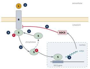
Our running example is a simplified version of how cells respond to cytokines, secreted proteins such as interleukins and interferons that coordinate immune responses (Figure 1.1).

A cytokine (the ligand, L) binds its receptor (R) at the cell surface. The ligand-bound receptor activates kinases of the JAK family that are associated with it.
STAT transcription factors (S) dock on the active receptor and are phosphorylated by JAK. Phosphorylated STAT (pSTAT) leaves the receptor and moves to the nucleus.
In the nucleus pSTAT binds the promoters of target genes. One of these encodes SOCS (suppressor of cytokine signaling).
SOCS protein binds the receptor and blocks further STAT activation. Because the output of the pathway inhibits its own input, the circuit is a negative feedback loop.

Figure 1.1: The cytokine–STAT–SOCS circuit. Numbers mark the six steps we model in this chapter: (1) ligand binding, (2) STAT recruitment to the ligand-bound receptor, (3) STAT activation, (4) release of pSTAT and its dephosphorylation, (5) induction of SOCS, and (6) SOCS feedback on the receptor.

We will build a model of this circuit one step at a time, adding the reactions for each step to the previous model and simulating as we go. The model leaves out many known details, such as STAT dimerization, the separate receptor chains, and transport into and out of the nucleus, some of which return in later chapters. Starting from a simple model makes each mechanism easier to follow, and the simple model already shows how feedback shapes the response.

1.3 Step 1: Ligand–receptor binding

Reactions and mass action

Binding of a ligand to its receptor is reversible:

\[ \mathrm{L} + \mathrm{R} \;\underset{k_\mathrm{off}}{\overset{k_\mathrm{on}}{\rightleftharpoons}}\; \mathrm{LR} \]

We treat this as two elementary reactions: binding, which consumes one L and one R and produces one LR, and unbinding, which does the reverse. The rate of each is given by the law of mass action, first stated by the Norwegian chemists Cato Guldberg and Peter Waage in the 1860s, which says that the rate of an elementary reaction is proportional to the product of the concentrations of its reactants. The proportionality constant is called the rate constant. Writing \([\mathrm{X}]\) for the concentration of species X, the two rates are

\[ v_1 = k_\mathrm{on}\,[\mathrm{L}]\,[\mathrm{R}], \qquad v_2 = k_\mathrm{off}\,[\mathrm{LR}]. \]

The units follow from the rate law. Rates have units of concentration per time, so the second-order constant \(k_\mathrm{on}\) has units of µM⁻¹ min⁻¹ and the first-order constant \(k_\mathrm{off}\) has units of min⁻¹. Mass action applies to elementary reactions, and it is a good description when molecules are well mixed and each reaction event requires a single encounter of its reactants. Later chapters consider what happens when these assumptions fail.

From reactions to differential equations

Each reaction changes the concentration of each species it involves: reactants are consumed and products are created. Binding lowers \([\mathrm{L}]\) and \([\mathrm{R}]\) and raises \([\mathrm{LR}]\); unbinding does the reverse. Adding up the contributions of all reactions to each species gives one ordinary differential equation per species:

\[ \begin{aligned} \frac{d[\mathrm{L}]}{dt} &= -k_\mathrm{on}[\mathrm{L}][\mathrm{R}] + k_\mathrm{off}[\mathrm{LR}],\\ \frac{d[\mathrm{R}]}{dt} &= -k_\mathrm{on}[\mathrm{L}][\mathrm{R}] + k_\mathrm{off}[\mathrm{LR}],\\ \frac{d[\mathrm{LR}]}{dt} &= +k_\mathrm{on}[\mathrm{L}][\mathrm{R}] - k_\mathrm{off}[\mathrm{LR}]. \end{aligned} \tag{1.1}\]

Once the reactions and rate laws are written down, the differential equations follow mechanically, which is why software such as BioNetGen can generate them for us.

The stoichiometry matrix

The bookkeeping in Equation 1.1 has a compact general form. Collect the concentrations in a vector \(\mathbf{X}\) and the reaction rates in a vector \(\mathbf{v}\). Then

\[ \frac{d\mathbf{X}}{dt} = \mathbf{S}\,\mathbf{v}(\mathbf{X}), \qquad \frac{d}{dt}\begin{pmatrix}[\mathrm{L}]\\ [\mathrm{R}]\\ [\mathrm{LR}]\end{pmatrix} = \begin{pmatrix}-1 & +1\\ -1 & +1\\ +1 & -1\end{pmatrix} \begin{pmatrix}k_\mathrm{on}[\mathrm{L}][\mathrm{R}]\\ k_\mathrm{off}[\mathrm{LR}]\end{pmatrix}, \tag{1.2}\]

where the stoichiometry matrix \(\mathbf{S}\) has one row per species and one column per reaction. Its entries are

\[ \begin{aligned} S_{ij} = {} & (\text{times species } i \text{ is a product of reaction } j)\\ & - (\text{times species } i \text{ is a reactant of reaction } j). \end{aligned} \]

Equation 1.2 holds for any reaction network; only \(\mathbf{S}\) and the rate laws in \(\mathbf{v}\) change from one network to another.

Conservation laws and equilibrium

Binding only moves molecules between free and bound forms. The total amounts of ligand and receptor are therefore constant:

\[ [\mathrm{L}] + [\mathrm{LR}] = L_0, \qquad [\mathrm{R}] + [\mathrm{LR}] = R_0, \]

where \(L_0\) and \(R_0\) are the total concentrations of ligand and receptor, free and bound. When the system starts with no complex, as here, they are the initial concentrations of L and R. These conservation laws appear as linear dependencies among the rows of \(\mathbf{S}\). Here the rows for L and R are both equal to minus the row for LR, so only one of the three equations is independent.

Consider what happens after a long time, when the system has reached equilibrium. Binding and unbinding then occur at the same rate (\(v_1 = v_2\)), so

\[ \frac{[\mathrm{L}][\mathrm{R}]}{[\mathrm{LR}]} = \frac{k_\mathrm{off}}{k_\mathrm{on}} \equiv K_D, \]

which defines the dissociation constant \(K_D\). Substituting the conservation laws gives a quadratic equation for the equilibrium amount of complex, whose physically meaningful root is

\[ [\mathrm{LR}]_\mathrm{eq} = \tfrac12\left[\, b - \sqrt{b^2 - 4L_0R_0}\,\right], \qquad b = L_0 + R_0 + K_D. \tag{1.3}\]

Solving the equations numerically

A model this small can be solved by hand, but the equations for realistic signaling networks are nonlinear and usually have no closed-form solution, so we integrate them numerically. The simplest scheme, forward Euler, takes small time steps,

\[ \mathbf{X}(t+\Delta t) \approx \mathbf{X}(t) + \Delta t\;\mathbf{S}\,\mathbf{v}(\mathbf{X}(t)). \]

In practice, reactions in a network often occur on very different time scales. When the fastest processes relax much more quickly than the dynamics of interest, the equations are stiff, meaning that simple methods like Euler’s need impractically small steps to remain stable. Production solvers such as CVODE adapt the step size and use implicit methods designed for stiff systems. BioNetGen and bngsim use CVODE for ODE simulation.

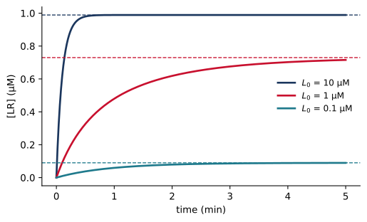
Figure 1.2 shows binding over time at three ligand concentrations, computed with bngsim from the BNGL model introduced in the next section. The code that produced it is shown above the figure. It loads the model, changes the initial ligand concentration L0, and runs an ODE simulation for each value.

model = bngsim.Model.from_bngl(model_path("ch01", "stat_step1_binding"))
sim = bngsim.Simulator(model, method="ode")

R0, KD = 1.0, 0.1
for L0 in [10, 1, 0.1]:
    model.set_param("L0", L0)
    model.reset()                      # back to initial conditions
    result = sim.run(t_span=(0, 5), n_points=501)
    line, = plt.plot(result.time, result.observables["LR"],
                     label=f"$L_0$ = {L0} µM")
    b = L0 + R0 + KD                   # equilibrium, from the formula
    LR_eq = (b - np.sqrt(b**2 - 4 * L0 * R0)) / 2
    plt.axhline(LR_eq, ls="--", lw=1, color=line.get_color())
model.set_param("L0", 10)              # restore default
plt.xlabel("time (min)")
plt.ylabel("[LR] (µM)")
plt.legend(loc="center right");

Figure 1.2: Ligand–receptor binding approaches equilibrium faster, and binds more receptors, at higher ligand concentration. Solid lines are numerical solutions; dashed lines are the equilibrium values from Equation 1.3. \(R_0 = 1\) µM, \(k_\mathrm{on} = 1\) µM⁻¹min⁻¹, \(k_\mathrm{off} = 0.1\) min⁻¹ (\(K_D = 0.1\) µM).

Given that at \(L_0 = 10\) µM the ligand is in large excess over both \(K_D\) and \(R_0\), one expects almost every receptor to be bound, and the simulation confirms this. Adding more ligand can increase the response only slightly, since the receptors are already nearly saturated. Binding is also faster at higher ligand concentration. Near equilibrium the complex relaxes at rate \(k_\mathrm{on}([\mathrm{L}] + [\mathrm{R}]) + k_\mathrm{off}\), which grows with the amount of free ligand.

1.4 Writing the model in BioNetGen

Here is the complete model file for ligand–receptor binding, models/ch01/stat_step1_binding.bngl:

begin model

begin parameters
  L0        10     # ligand (uM)
  R0        1      # receptor (uM)
  kon       1      # binding (1/uM/min)
  koff      0.1    # unbinding (1/min)
end parameters

begin molecule types
  L
  R
  LR
end molecule types

begin species
  L    L0
  R    R0
end species

begin observables
  Molecules Lfree   L
  Molecules Rfree   R
  Molecules LR      LR
end observables

begin reaction rules
  # Ligand binds receptor
  LRbind: L + R <-> LR kon, koff
end reaction rules

end model

generate_network({overwrite=>1})
simulate({method=>"ode",t_end=>2,n_steps=>200})

A BNGL file has a model section, between begin model and end model, and an actions section after it.

parameters names every quantity that appears in the model, with its value. Lines starting with # are comments.
molecule types declares every kind of species. In this chapter species have no internal structure, so each is just a name. Chapter 2 gives molecules binding sites and states.
species lists the species present at the start and their initial amounts. Here these are given by the parameters L0 and R0. Species not listed start at zero.
observables defines the quantities to report. Molecules LR LR reports the amount of species LR under the name LR.
reaction rules lists the reactions. <-> marks a reversible reaction, followed by the forward and reverse rate constants. The optional label (LRbind:) names the rule.
The actions tell BioNetGen what to do with the model: generate_network builds the list of species and reactions, and simulate integrates the ODEs and writes the observables to a .gdat file.

You can run the model in three ways. In VS Code with the BioNetGen extension, open the file and click the run button, and the results open in a plot viewer. In BNG Playground, paste the file into the editor and click Run. From Python, load the model with bngsim, as in the code for Figure 1.2:

model = bngsim.Model.from_bngl("models/ch01/stat_step1_binding.bngl")
sim = bngsim.Simulator(model, method="ode")
model.reset()
result = sim.run(t_span=(0, 20), n_points=101)
result.observables["LR"]          # time course of LR

Model.from_bngl uses BioNetGen to generate the network but does not run the file’s actions, so the simulation is controlled entirely from Python. Parameters are changed on the model with model.set_param, and model.reset() returns the species to their initial amounts. It is important to note that a run starts from the model’s current state, which is wherever the previous run ended, so model.reset() should be called before each run.

1.5 Building the circuit step by step

Each of the remaining steps adds a few reactions to the model. The model files stat_step2_recruit.bngl through stat_step6_feedback.bngl are cumulative, and lines added at each step are marked # new. Below we show only the new lines.

Step 2: STAT binds the ligand-bound receptor

\[ \mathrm{LR} + \mathrm{S} \rightleftharpoons \mathrm{LRS} \]

STAT binds the ligand-bound receptor LR but never free R. Since the model contains no reaction in which free receptor recruits STAT, ligand binding is required for STAT recruitment. Every new species needs a molecule type, and species present at the start also need an initial amount.

begin parameters
  S0        10     # STAT (uM)
  kSon      1      # STAT binding (1/uM/min)
  kSoff     1      # STAT unbinding (1/min)
end parameters
begin molecule types
  S
  LRS
end molecule types
begin species
  S    S0
end species
begin observables
  Molecules Sfree   S
  Molecules LRS     LRS
end observables
begin reaction rules
  # STAT binds ligand-bound receptor
  Sbind: LR + S <-> LRS kSon, kSoff
end reaction rules

Step 3: Receptor-bound STAT is activated

\[ \mathrm{LRS} \xrightarrow{\;k_\mathrm{act}\;} \mathrm{LRS_p} \]

The receptor-associated kinase phosphorylates the docked STAT. This is a first-order, irreversible reaction with rate \(v = k_\mathrm{act}[\mathrm{LRS}]\).

begin parameters
  kact      1      # STAT activation (1/min)
end parameters
begin molecule types
  LRSp
end molecule types
begin observables
  Molecules LRSp    LRSp
  Molecules pSTAT   LRSp
end observables
begin reaction rules
  # Receptor-associated kinase activates STAT
  Sact: LRS -> LRSp kact
end reaction rules

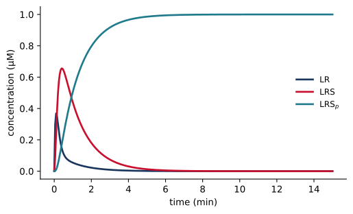
Consider what this model implies. Nothing in it releases activated STAT from the receptor, so one would expect every receptor to end up trapped as LRS_p, having activated a single STAT. The simulation confirms this expectation (Figure 1.3).

Code

model = bngsim.Model.from_bngl(model_path("ch01", "stat_step3_activate"))
sim = bngsim.Simulator(model, method="ode")
model.reset()
r = sim.run(t_span=(0, 15), n_points=301)
for name, label in [("LR", "LR"), ("LRS", "LRS"), ("LRSp", "LRS$_p$")]:
    plt.plot(r.time, r.observables[name], label=label)
plt.xlabel("time (min)")
plt.ylabel("concentration (µM)")
plt.legend();

Figure 1.3: With activation but no release (step 3), every receptor ends up as LRS_p.

Step 4: Activated STAT is released and deactivated

\[ \mathrm{LRS_p} \xrightarrow{\;k_\mathrm{diss}\;} \mathrm{LR} + \mathrm{S_p}, \qquad \mathrm{S_p} \xrightarrow{\;k_\mathrm{dephos}\;} \mathrm{S} \]

Releasing pSTAT frees the receptor to activate another STAT, so one receptor can now activate many. A phosphatase returns free pSTAT to the inactive pool.

begin parameters
  kdiss     1      # pSTAT release (1/min)
  kdephos   0.1    # pSTAT dephosphorylation (1/min)
end parameters
begin molecule types
  Sp
end molecule types
begin observables
  Molecules Sp      Sp
  Molecules pSTAT   LRSp Sp
end observables
begin reaction rules
  # Activated STAT dissociates
  Srelease: LRSp -> LR + Sp kdiss
  # Phosphatase deactivates free STAT
  Sdephos: Sp -> S kdephos
end reaction rules

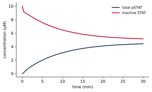
Total pSTAT now rises to a steady state set by the balance between activation and dephosphorylation (Figure 1.4). A steady state differs from the binding equilibrium above. At equilibrium every reaction is balanced by its reverse, whereas here STAT cycles continuously through phosphorylation, release, and dephosphorylation, and the amounts stay constant only because these irreversible steps run at equal rates. Maintaining such a cycle requires a source of energy, which in cells is the ATP consumed by the kinase. The observable pSTAT sums all species that contain phosphorylated STAT. Its definition lists them by name, LRSp Sp, a chore we return to in Chapter 2.

Code

model = bngsim.Model.from_bngl(model_path("ch01", "stat_step4_release"))
sim = bngsim.Simulator(model, method="ode")
model.reset()
r = sim.run(t_span=(0, 30), n_points=301)
plt.plot(r.time, r.observables["pSTAT"], label="total pSTAT")
plt.plot(r.time, r.observables["Sfree"], label="inactive STAT")
plt.xlabel("time (min)")
plt.ylabel("concentration (µM)")
plt.legend();

Figure 1.4: With release and dephosphorylation (step 4), pSTAT reaches a steady state.

Step 5: pSTAT induces SOCS expression

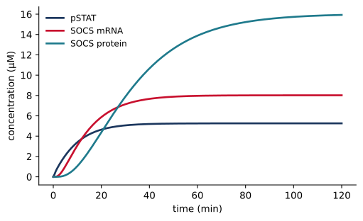
In step 5, pSTAT binds the SOCS promoter (G), the bound promoter is transcribed into SOCS mRNA, and the mRNA is translated into SOCS protein. Both mRNA and protein are degraded.

begin parameters
  G0        1      # SOCS gene promoter (uM)
  kGon      1      # pSTAT-promoter binding (1/uM/min)
  kGoff     1      # pSTAT-promoter unbinding (1/min)
  ktx       1      # transcription (1/min)
  kmdeg     0.1    # mRNA degradation (1/min)
  ktl       0.1    # translation (1/min)
  kSOCSdeg  0.05   # SOCS degradation (1/min)
end parameters
begin molecule types
  G
  GSp
  mSOCS
  SOCS
end molecule types
begin species
  G    G0
end species
begin observables
  Molecules mSOCS   mSOCS
  Molecules SOCS    SOCS
  Molecules pSTAT   LRSp Sp GSp
end observables
begin reaction rules
  # pSTAT binds the SOCS promoter
  Gbind: Sp + G <-> GSp kGon, kGoff
  # Bound promoter is transcribed
  Transcribe: GSp -> GSp + mSOCS ktx
  # mRNA degradation
  mRNAdeg: mSOCS -> 0 kmdeg
  # Translation
  Translate: mSOCS -> mSOCS + SOCS ktl
  # SOCS protein degradation
  SOCSdeg: SOCS -> 0 kSOCSdeg
end reaction rules

This step introduces synthesis and degradation reactions. In a synthesis reaction such as GSp -> GSp + mSOCS, a species appears on both sides; it acts as a template and is not consumed, so the rate is proportional to its amount. In a degradation reaction such as SOCS -> 0, the product 0 indicates that the molecule is removed. The rate constants of these reactions are first order.

SOCS now accumulates, but it does not yet act on anything, so pSTAT is essentially unchanged (Figure 1.5).

Code

model = bngsim.Model.from_bngl(model_path("ch01", "stat_step5_transcribe"))
sim = bngsim.Simulator(model, method="ode")
model.reset()
r = sim.run(t_span=(0, 120), n_points=241)
for name, label in [("pSTAT", "pSTAT"), ("mSOCS", "SOCS mRNA"), ("SOCS", "SOCS protein")]:
    plt.plot(r.time, r.observables[name], label=label)
plt.xlabel("time (min)")
plt.ylabel("concentration (µM)")
plt.legend();

Figure 1.5: With SOCS expression but no feedback (step 5), SOCS mRNA and protein accumulate while pSTAT is unaffected.

Step 6: SOCS closes the feedback loop

\[ \mathrm{LR} + \mathrm{SOCS} \rightleftharpoons \mathrm{LR{\cdot}SOCS} \]

SOCS competes with STAT for the ligand-bound receptor. The complex LR·SOCS cannot recruit STAT, so as SOCS accumulates, pSTAT production falls. This reaction completes the feedback loop:

\[ \text{pSTAT} \;\longrightarrow\; \text{SOCS} \;\dashv\; \text{receptor} \;\longrightarrow\; \text{pSTAT}. \]

begin parameters
  kSOCSon   1      # SOCS-receptor binding (1/uM/min)
  kSOCSoff  0.01   # SOCS-receptor unbinding (1/min)
end parameters
begin molecule types
  LRSOCS
end molecule types
begin observables
  Molecules LRSOCS  LRSOCS
end observables
begin reaction rules
  # SOCS binds ligand-bound receptor, blocking STAT binding
  SOCSbind: LR + SOCS <-> LRSOCS kSOCSon, kSOCSoff
end reaction rules

1.6 Negative feedback turns a sustained signal into a pulse

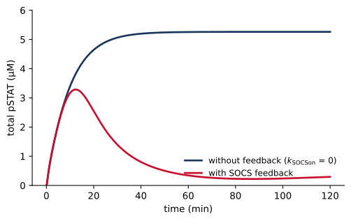
Figure 1.6 compares the full model with the same model when SOCS cannot bind the receptor (\(k_\mathrm{SOCSon} = 0\)). The model file runs both simulations itself, using the action setParameter between them. Here we do the same from Python.

model = bngsim.Model.from_bngl(model_path("ch01", "stat_step6_feedback"))
sim = bngsim.Simulator(model, method="ode")

for kSOCSon, label in [(0, "without feedback ($k_\\mathrm{SOCSon}$ = 0)"),
                       (1, "with SOCS feedback")]:
    model.set_param("kSOCSon", kSOCSon)
    model.reset()
    r = sim.run(t_span=(0, 120), n_points=1201)
    plt.plot(r.time, r.observables["pSTAT"], label=label)
plt.xlabel("time (min)")
plt.ylabel("total pSTAT (µM)")
plt.ylim(0, 6)
plt.legend(loc="lower right");

Figure 1.6: Negative feedback turns a sustained response into a pulse. Without feedback, pSTAT rises to a high plateau. With feedback, it peaks and then falls to a much lower adapted level, even though ligand is still present.

Following the addition of ligand, receptors bind ligand within seconds and begin to activate STAT, and pSTAT rises along the same curve whether or not SOCS can act, since no SOCS has yet been made. In the full model, SOCS accumulates over the next 10 to 20 minutes and binds the active receptors, and pSTAT falls to a low level even though ligand is still present, a behavior called adaptation. The delay before the feedback acts comes from the intervening steps, in which pSTAT must bind the promoter, mRNA must accumulate, and SOCS protein must build up to levels comparable to the receptor.

The pulse can be described by three properties: the time of the peak, the height of the peak, and the adapted level that pSTAT settles to. Each depends on the parameters in a different way. The exercises at the end of the chapter ask you to predict these dependencies, and a later chapter on model analysis develops tools to study them systematically.

1.7 The complete network and its limits

Table 1.1 lists the complete model. Eleven reaction lines in BNGL define 15 reactions among 12 species, since four of the reactions are reversible. BioNetGen generates the stoichiometry matrix and the 12 ODEs from this list, and writes the network to a .net file that you can inspect.

Table 1.1: The cytokine–STAT–SOCS reaction network.

Step	Reaction	Rate constants
1	L + R \(\rightleftharpoons\) LR	\(k_\mathrm{on}\), \(k_\mathrm{off}\)
2	LR + S \(\rightleftharpoons\) LRS	\(k_\mathrm{Son}\), \(k_\mathrm{Soff}\)
3	LRS \(\to\) LRS_p	\(k_\mathrm{act}\)
4	LRS_p \(\to\) LR + S_p	\(k_\mathrm{diss}\)
	S_p \(\to\) S	\(k_\mathrm{dephos}\)
5	S_p + G \(\rightleftharpoons\) GS_p	\(k_\mathrm{Gon}\), \(k_\mathrm{Goff}\)
	GS_p \(\to\) GS_p + mSOCS	\(k_\mathrm{tx}\)
	mSOCS \(\to\) 0	\(k_\mathrm{mdeg}\)
	mSOCS \(\to\) mSOCS + SOCS	\(k_\mathrm{tl}\)
	SOCS \(\to\) 0	\(k_\mathrm{SOCSdeg}\)
6	LR + SOCS \(\rightleftharpoons\) LR·SOCS	\(k_\mathrm{SOCSon}\), \(k_\mathrm{SOCSoff}\)

The model makes strong simplifying assumptions, and relaxing them exposes two limitations of the approach in this chapter.

First, every species had to be named by hand: L, LR, LRS, LRS_p, LR·SOCS, and so on. Suppose SOCS could also bind receptors that already carry STAT, or ligand could dissociate from any receptor complex. Each such change creates new complexes, and each complex needs its own name and its own copy of every reaction it takes part in. For real signaling proteins, with many binding sites and modification sites, the number of possible complexes grows combinatorially. Chapter 2 introduces rules that act on structured molecules, so that the network is generated automatically.

Second, ODEs treat concentrations as continuous and deterministic. A cell may contain only one or two copies of the SOCS gene and a handful of mRNA molecules. At such small numbers the random timing of individual reactions matters, and genetically identical cells respond differently. The same reaction network can be simulated stochastically, which is the subject of Chapter 3.

1.8 Summary

A reaction network model consists of species, reactions, rate laws, and initial conditions.
Mass-action rate laws turn the network into ODEs, which have the general form \(d\mathbf{X}/dt = \mathbf{S}\,\mathbf{v}(\mathbf{X})\).
Conservation laws reduce the number of independent equations. Simple models can be solved analytically; realistic ones are integrated numerically with stiff solvers.
BNGL describes the network directly. BioNetGen and bngsim generate and integrate the equations.
Building the cytokine–STAT–SOCS circuit one step at a time shows what each mechanism contributes. Negative feedback through SOCS turns a sustained response into an adaptive pulse.

1.9 Exercises

These exercises are also available as a printable worksheet in the course repository.

Binding equilibrium. Using stat_step1_binding.bngl, compute \([\mathrm{LR}]_\mathrm{eq}\) from Equation 1.3 for \(L_0\) = 0.1, 1, and 10 µM, and compare with simulations run to \(t = 20\) min. Above roughly what ligand concentration are almost all receptors bound?
Tuning the pulse. For each of L0, kact, kdiss, kdephos, ktl, and kSOCSdeg, predict whether doubling the parameter raises, lowers, or leaves unchanged the time of the peak, the peak height, and the adapted level of pSTAT. Then test your predictions with stat_step6_feedback.bngl, simulating to \(t = 600\) min so that pSTAT settles. Which parameter changes only the adapted level, and why? Why does doubling L0 have almost no effect, and does it matter at \(L_0 = 0.1\) µM?
No phosphatase. In stat_step4_release.bngl, set kdephos to 0. Predict, then simulate, the long-time value of total pSTAT. What sets this value?
Toward rules. Suppose SOCS can also bind receptors that carry unphosphorylated STAT (LRS). Write the new reaction in the notation of this chapter, and list the other reactions that the new complex needs. How many new species would you need if SOCS could also bind LRS_p?

1.10 Further reading

Faeder et al. (2009) is a thorough introduction to BNGL and the BioNetGen software. Sekar and Faeder (2012) is a self-contained tutorial on rule-based modeling of signal transduction. Harris et al. (2016) describes features added in BioNetGen 2.2.