Most models of signaling are assembled from a small number of recurring mechanisms: binding, modification by enzymes, synthesis, degradation, and the formation of larger complexes. Chapter 2 introduced the syntax of rules, and this chapter shows how to write rules for each of these mechanisms, what reactions BioNetGen generates from them, and where the generated network can differ from what the modeler intended. Each section is built around a small model in models/ch04/, and for each one we look at the reactions BioNetGen produces. Reading the generated network is the most reliable way to check a rule, and new modelers should make it a habit. The chapter closes with a list of common mistakes that are hard to spot without reading the generated network.
NoteLearning goals
After this chapter you should be able to:
write rules for binding, including binding of identical molecules and of molecules with several identical sites, and predict the statistical factors BioNetGen applies;
use context to make a rate depend on the state of another site;
model enzymatic modification with an explicit mechanism or with a Michaelis–Menten rate law, and choose between them;
write rules for synthesis and degradation, including degradation of a molecule that is part of a complex;
define rate laws with functions of observables;
write rules for the formation of chains and rings, and limit the size of the network they generate.
4.1 Reading the generated network
Every rule in this chapter is checked the same way. BioNetGen generates the network, and we list the reactions it contains, written out with the full species on each side and the rate law of each reaction. The listing comes from the .net file that generate_network writes, which can also be opened directly in any text editor. The rate laws in this listing contain the statistical factors that BioNetGen derives from the structure of the molecules, and these factors are the main subject of the next section.
4.2 Binding
Identical partners
Consider two molecules of the same type that bind each other through a single site to form a dimer:
The rate constant of the forward reaction is 0.5*kf, not kf. The factor of one half accounts for the fact that the two reactants are identical. In a system of \(N\) molecules there are \(N(N-1)/2\) distinct pairs, not \(N^2\), and the factor in the generated reaction makes the deterministic and stochastic descriptions consistent with this count. The ODE for the dimer is thus
The practical consequence concerns rate constants taken from the literature. If a published model writes the dimerization rate as \(k[\mathrm{A}]^2\), the rule must use 2*k to reproduce it. It is important to note that conventions differ among papers and software packages, so a rate constant for a symmetric reaction should never be copied without checking which convention was used.
Multiple identical sites
The opposite situation arises when one molecule has several identical sites for a partner. In bivalent.bngl, molecule A has two equivalent sites for B, declared by repeating the component name, A(b,b). A single rule describes binding at either site:
Free A binds B at rate 2*kon, since either of its two empty sites can be used, while A with one site filled binds a second B at rate kon. Likewise, the complex with two bound B molecules releases one at rate 2*koff. These factors follow from counting the ways a rule can be applied to a species, and BioNetGen computes them automatically.
Cooperativity through context
Binding at one site often changes binding at another. In cooperative.bngl, a receptor has two sites, a and b, and ligand binds site b ten times faster when site a is already occupied:
The context R(a,b) in the first rule restricts it to receptors with both sites empty, and R(a!+,b) restricts the second rule to receptors with site a filled. The generated network shows a consequence that is easy to miss. The reverse of each rule applies the same context as the forward direction, so ligand bound at site a can leave only while site b is empty. If both sites can release their ligand independently, the unbinding reactions must be written as separate rules without that context, as we did for STAT in Chapter 2. When the sites can be filled in either order, however, the four binding rate constants cannot be chosen independently, since both orders lead to the same doubly occupied receptor. Chapter 8 derives this constraint and shows how energy patterns satisfy it automatically.
4.3 Enzymatic modification
A kinase that phosphorylates a substrate can be modeled at two levels of detail. The explicit mechanism follows the elementary steps, binding of enzyme and substrate followed by catalysis and release:
When the enzyme–substrate complex reaches a quasi-steady state quickly compared with the depletion of substrate, the rate of phosphorylation takes the familiar Michaelis–Menten form, \[
v = \frac{k_\mathrm{cat}[\mathrm{E}]_T[\mathrm{S}]}{K_m + [\mathrm{S}]},
\tag{4.1}\] where \([\mathrm{E}]_T\) is the total enzyme, free and bound, \([\mathrm{S}]\) is the free substrate, and \(K_m = (k_\mathrm{off} + k_\mathrm{cat})/k_\mathrm{on}\). The classical form of the approximation also replaces free by total substrate, which is valid only when little substrate is bound to enzyme, that is, when \([\mathrm{E}]_T \ll [\mathrm{S}]_T + K_m\)(Borghans et al. 1996). BNGL provides a Michaelis–Menten rate law as the built-in MM(kcat,Km):
# consumed. MM treats the amounts matching the two patterns as totals.MMcat: S2(Y~0) + E2() -> S2(Y~P) + E2() MM(kcat,Km)
The substrate is written first and the enzyme second, and the enzyme appears on both sides of the rule, since it is not consumed. MM treats the amounts of the species that match the two reactant patterns as the totals \([\mathrm{S}]_T\) and \([\mathrm{E}]_T\), and it does not assume that they are nearly equal to the free amounts. It computes the free substrate from \[
[\mathrm{S}] = \tfrac12\left[\left([\mathrm{S}]_T - K_m - [\mathrm{E}]_T\right)
+ \sqrt{\left([\mathrm{S}]_T - K_m - [\mathrm{E}]_T\right)^2 + 4K_m[\mathrm{S}]_T}\,\right]
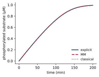
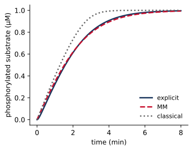
\] and uses this value in Equation 4.1. This is the total quasi-steady-state approximation of Borghans et al. (1996), which accounts for the substrate held by the enzyme and remains accurate at much higher enzyme concentrations (Tzafriri 2003). When \([\mathrm{E}]_T \ll [\mathrm{S}]_T + K_m\), free and total substrate are nearly equal, and MM reduces to the classical form. Figure 4.1 compares the explicit mechanism, MM, and the classical form.
Code
model = bngsim.Model.from_bngl(model_path("ch04", "enzyme"))sim = bngsim.Simulator(model, method="ode")kcat, Km, S0 = (model.get_param(p) for p in ("kcat", "Km", "S0"))def classical(t, E0):# Integrate dSp/dt = kcat*E0*S/(Km + S) with S = S0 - Sp (Euler, fine grid) sp = np.zeros_like(t)for i inrange(1, len(t)): S = S0 - sp[i-1] sp[i] = sp[i-1] + (t[i] - t[i-1]) * kcat * E0 * S / (Km + S)return spdef t_half(t, y):return np.interp(S0 /2, y, t)half = {}for E0, t_end in [(0.01, 200), (0.5, 8)]: model.set_param("E0", E0) model.reset() r = sim.run(t_span=(0, t_end), n_points=4001) cl = classical(r.time, E0) half[E0] = {"explicit": t_half(r.time, r.observables["Sp_explicit"]),"MM": t_half(r.time, r.observables["Sp_MM"]),"classical": t_half(r.time, cl)} fig, ax = plt.subplots(figsize=(4.2, 3.2)) ax.plot(r.time, r.observables["Sp_explicit"], color="#1B365D", label="explicit") ax.plot(r.time, r.observables["Sp_MM"], "--", color="#C8102E", label="MM") ax.plot(r.time, cl, ":", color="0.4", label="classical") ax.set_xlabel("time (min)") ax.set_ylabel("phosphorylated substrate (µM)") ax.legend(loc="lower right") plt.show()model.set_param("E0", 0.01)
(a)
(b)
Figure 4.1: Phosphorylation by a kinase described by an explicit binding–catalysis mechanism (solid), by the MM rate law (dashed), and by the classical Michaelis–Menten form (dotted), with 1 µM substrate. (a) Scarce enzyme, 0.01 µM: the three agree. (b) Abundant enzyme, 0.5 µM: the classical form runs too fast, while MM remains close to the explicit mechanism.
The three descriptions agree closely when the enzyme is scarce. With enzyme at half the concentration of substrate, the classical form overestimates the rate, since it counts substrate held by the enzyme as free, and it predicts that half of the substrate is phosphorylated in 1.28 min rather than 1.57 min. MM gives 1.52 min. The rate law is more economical, since it introduces no enzyme–substrate complexes, and its two parameters, \(k_\mathrm{cat}\) and \(K_m\), are the ones usually reported by enzymologists. The explicit mechanism, on the other hand, is required whenever the enzyme–substrate complex matters in its own right: when substrates compete for the enzyme, when the enzyme is abundant enough to be sequestered, or when the complex has other interactions, as a receptor-bound STAT does.
The rate law also hides a trap, which appeared while the models for this chapter were being written. In the first version of enzyme.bngl, the same kinase molecule was used for both the explicit and the Michaelis–Menten rules. The explicit rules tied up most of the kinase in enzyme–substrate complexes. The MM rule counted as its total enzyme only the kinase that matched its enzyme pattern, which excluded the kinase held in these complexes, and the Michaelis–Menten reaction ran about five times too slowly. The model file now uses a separate kinase for each mechanism. The general lesson is that an enzyme described by an MM rate law should not also participate in explicit binding rules for the same reaction.
4.4 Making and removing molecules
Synthesis and degradation were introduced in Chapter 1. Synthesis from nothing, 0 -> A(), describes production at a constant rate, for example from a gene that is not part of the model, and synthesis from a template, G(s!+) -> G(s!+) + mRNA(), describes production at a rate proportional to the amount of the template. Degradation needs more care when the molecule being degraded can be part of a complex. degradation.bngl contains three pairs of bound molecules and three ways of writing a degradation rule:
beginreactionrules# Deletes the whole complex that contains A, including B DegA: A() ->0 kdeg# Deletes only C; its partner D is released DegC: C() ->0 kdeg DeleteMolecules# Writes the outcome explicitly: E is removed and F is released DegE: E(f!1).F(e!1) -> F(e) kdegendreactionrules
The first rule removes not only A but its partner B, since by default a molecule deleted by a rule takes the entire complex that contains it. The keyword DeleteMolecules in the second rule changes this behavior, so that only C is removed and its partner D is released. The third rule gives the same result as the second by writing the product explicitly. Which behavior is correct depends on the biology. Degradation of a receptor by internalization may reasonably take its bound ligand with it, while proteolysis of one subunit of a complex usually releases the others.
4.5 Rate laws from functions
Sometimes a process is not worth modeling at the level of elementary reactions, either because its mechanism is unknown or because its details are not the subject of the model. BNGL allows the rate of a rule to be any mathematical function of parameters and observables, defined in a functions block. In hill.bngl, transcription of a target gene is a Hill function of the amount of phosphorylated STAT, which replaces the explicit promoter binding of Chapter 1:
The function fTx() is evaluated as the simulation proceeds, using the current value of the observable pSTAT. A function used as a rate law takes the place of the rate constant, so the rate of each generated reaction is the value of the function multiplied by the amounts of the reactants, just as for mass action. Here the rule has no reactants, and the rate of mRNA synthesis is thus fTx() itself. With a Hill coefficient \(n = 2\) and half-maximal pSTAT \(K\), the rate rises steeply as pSTAT passes \(K\), mimicking cooperative binding of STAT dimers to the promoter without modeling the dimers.
Lumped rate laws of this kind should be used deliberately. A Hill function fitted to a dose–response curve can reproduce the curve without saying anything about the mechanism that produced it, and it cannot predict how the response changes when the mechanism is perturbed, for example by a mutation that prevents dimerization. A useful rule of thumb is to use explicit mechanisms for the parts of a system that are the subject of the study, and lumped rate laws only for the parts that are not.
4.6 Chains, rings, and the size of the network
When molecules have more than one binding site, they can form chains and rings of any length. The classic example in immune signaling is the crosslinking of receptors by multivalent ligands. aggregation.bngl contains a ligand with two sites and a receptor with two sites, with one rule for binding between complexes and one for closing a ring:
Bind: L(r) + R(l) <-> L(r!1).R(l!1) kon, koff# the reverse opens a ring without splitting the complexClose: L(r).R(l) <-> L(r!1).R(l!1) kring, koff
The rule Close has a single reactant pattern, L(r).R(l), in which the dot requires the ligand and the receptor to be in the same complex without requiring a bond between them. It therefore describes binding between a free ligand site and a free receptor site anywhere in one complex, which closes a chain of any length into a ring, and it is a unimolecular reaction with rate constant kring in units of inverse time. In contrast, the rule Bind has two reactant patterns separated by +, and BioNetGen applies it only to sites on different complexes. The distinction matters because the rate of ring closure, which depends on the flexibility and geometry of the complex, has no relation to the rate of binding between molecules in solution. Our model gives every ring the same kring, although a real chain closes at a rate that depends on its length.
The same distinction applies in reverse. The reverse of Bind breaks a bond only when the two products are separate complexes, and the reverse of Close breaks a bond only when the product remains a single complex, which is the case for a bond in a ring. Each bond in the network is thus broken by exactly one of the two rules, and BioNetGen enforces this by checking that the products of each reaction match the + or . written in the rule. Without the reverse of Close, rings could never open, and the model would slowly convert every molecule into rings. Since only a ligand end and a receptor end can close, only chains with equal numbers of ligands and receptors form rings.
Without a limit, the rule Bind generates chains of every length, and network generation never finishes. The option max_agg in the generate_network action caps the number of molecules in any complex. Table 4.1 shows how the network grows as the cap is raised.
Code
import pandas as pd, tempfile, os, resrc = model_path("ch04", "aggregation").read_text()# A ring is a species with no free site, r or l, on any molecule.rows = []for max_agg in [2, 4, 6, 8, 10]:with tempfile.TemporaryDirectory() as d: path = os.path.join(d, "aggregation.bngl")open(path, "w").write(src.replace("max_agg=>4", f"max_agg=>{max_agg}")) m = bngsim.Model.from_bngl(path, cache=False) rings = [sp for sp in m.species_names ifnot re.search(r"[rl][,)]", sp)] rows.append({"max_agg": max_agg, "species": m.n_species,"reactions": m.n_reactions, "rings": len(rings)})pd.DataFrame(rows).set_index("max_agg")
Table 4.1: Size of the network generated from aggregation.bngl as a function of max_agg, the largest complex allowed, and the number of distinct rings it contains.
species
reactions
rings
max_agg
2
4
4
1
4
8
16
2
6
12
34
3
8
16
60
4
10
20
92
5
The number of reactions grows faster than the number of species, since each new chain can react with every existing one. A cap on complex size is only justified when larger complexes are rare, which should be checked by simulating with a larger cap and confirming that the results do not change. When large aggregates are important, as they are in the activation of immunoreceptors, the network becomes too large to generate, and network-free simulation is the method of choice.
4.7 Common mistakes
The following mistakes are easy to make and hard to detect from simulation results alone.
Ignoring the symmetry factor. A rule for binding of identical molecules generates a reaction with half the written rate constant. Check the convention of any rate constant taken from the literature.
Missing context. A rule without context applies to every species that matches it, including complexes the modeler did not have in mind. Read the generated network for unintended reactions, as in Chapter 2, where removing one context from the ligand rule added reactions for every receptor complex.
Context in the reverse direction. A reversible rule applies its context in both directions. When the forward and reverse reactions should have different context, write them as two rules.
Deleting whole complexes. A degradation rule removes the entire complex containing the deleted molecule unless DeleteMolecules is given or the products are written explicitly.
Mixing explicit and lumped descriptions of the same enzyme. An MM rate law treats the amount of enzyme matching its pattern as the total enzyme, so an enzyme that also binds substrate through explicit rules will be undercounted.
Counting the wrong thing. A Molecules observable counts matches and a Species observable counts complexes. A function of an observable inherits this difference.
Inconsistent units. Rate constants and initial amounts must use the same units, either concentrations or molecule numbers, as discussed in Chapter 3.
4.8 Summary
Reading the reactions BioNetGen generates is the most reliable way to check that a rule does what was intended.
BioNetGen applies statistical factors automatically: one half for binding of identical molecules, and integer factors for molecules with several identical sites.
Context makes rates depend on the state of other sites, and it applies in both directions of a reversible rule.
Enzymatic modification can be modeled explicitly or with the MM rate law, which uses the total quasi-steady-state approximation. It agrees with the explicit mechanism, and with the classical Michaelis–Menten form, when the enzyme is scarce, and it remains accurate at higher enzyme concentrations than the classical form.
Degradation removes the whole complex unless DeleteMolecules is used or the products are given explicitly.
Rate laws can be functions of observables, which is useful for lumping processes that are not the subject of a model.
Rules for multivalent binding generate chains and rings of unbounded size. max_agg limits network generation, and network-free simulation avoids it.
4.9 Exercises
Symmetry. Write a model in which two molecules of A bind through two distinct sites, A(x,y), with x binding y. Compare the generated network with homodimer.bngl. Which reactions have statistical factors, and why?
Cooperativity. Modify cooperative.bngl so that either site can be occupied first and ligand can leave either site at any time. How many rules do you need? Plot the fraction of receptors with both sites filled as a function of ligand concentration for kon2 = 0.1, 1, and 10. Do your rate constants satisfy the cycle constraint of Section 8.1?
When does Michaelis–Menten fail? In enzyme.bngl, vary E0 from 0.001 to 1 µM and measure the time for half of the substrate to be phosphorylated by each mechanism. Explain where and why the two begin to disagree.
Degradation. Add a degradation rule for SOCS to stat_rbm1_rules.bngl from Chapter 2 that degrades SOCS whether it is free or bound to the receptor. Should the receptor be released or degraded with it? Write both versions and compare the adapted level of pSTAT.
Capping aggregation. Simulate aggregation.bngl with max_agg = 4, 6, and 8, and plot the observables Ring2 and Ring4 over time. Is a cap of 4 adequate for these parameters? How would you decide? What happens to the rings if Close is made irreversible?
4.10 Further reading
Sekar and Faeder (2012) contains an extensive library of example rules for signaling mechanisms, from binding at the membrane to gene regulation. Faeder et al. (2009) describes the syntax of rules, rate laws, and network generation options in detail.
Borghans, J. A. M., R. J. de Boer, and L. A. Segel. 1996. “Extending the Quasi-Steady State Approximation by Changing Variables.”Bulletin of Mathematical Biology 58 (1): 43–63. https://doi.org/10.1007/BF02458281.
Faeder, James R., Michael L. Blinov, and William S. Hlavacek. 2009. “Rule-Based Modeling of Biochemical Systems with BioNetGen.”Methods in Molecular Biology 500: 113–67. https://doi.org/10.1007/978-1-59745-525-1_5.
Sekar, John A. P., and James R. Faeder. 2012. “Rule-Based Modeling of Signal Transduction: A Primer.”Methods in Molecular Biology 880: 139–218. https://doi.org/10.1007/978-1-61779-833-7_9.