In Chapter 1 every species in the cytokine–STAT–SOCS model had a name, such as L, LR, LRS, LRSp, and LR·SOCS. Naming species by hand works for twelve species but fails once the model includes what is known about the molecules involved, because signaling proteins have many binding and modification sites and the number of ways those sites can be combined grows combinatorially. Rule-based modeling, developed in the early 2000s to address this problem (Blinov et al. 2004; Hlavacek et al. 2006), represents molecules as structured objects with sites and states, and writes each interaction as a rule that mentions only the parts of the molecules that matter. BioNetGen then generates the reaction network from the rules.
NoteLearning goals
After this chapter you should be able to:
explain why multi-site proteins lead to combinatorial complexity;
represent molecules with components, states, and bonds in BNGL;
read and write patterns, and use them to define observables;
write reaction rules and predict which reactions a rule generates;
read a contact map and a rule diagram, and distinguish what a rule changes from its context;
describe how BioNetGen generates a network from rules, and when network-free simulation is needed instead.
2.1 Signaling proteins have many interaction sites
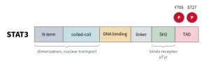
Figure 2.1 shows the domain structure of STAT3. Its SH2 domain binds phosphotyrosines on activated receptors. Tyrosine 705, near the C terminus, is phosphorylated by JAK, and the phosphorylated tyrosine of one STAT binds the SH2 domain of another to form an active dimer. Serine 727, in the transactivation domain, is phosphorylated separately and modulates transcriptional activity. The N-terminal and coiled-coil regions mediate further interactions and nuclear transport, and the DNA-binding domain binds promoters.
Figure 2.1: Domain structure of STAT3. Each domain or modification site is a separate place where the protein can interact or change state.
The receptor and JAK have their own sets of sites, as does nearly every signaling protein, and these sites can be occupied or modified in combination. Consider a protein with \(n\) sites, each of which can be modified independently. Such a protein has \(2^n\) possible states, and since a complex combines the states of all its parts, the number of possible complexes grows faster still. This growth is called combinatorial complexity. In a model of the ErbB receptor family with its known binding partners, a single ErbB1 homodimer can take more than \(5\times
10^{10}\) distinct states, and an ErbB1–ErbB3 heterodimer more than \(3.8\times
10^9\), far more than could be named individually (Creamer et al. 2012).
However, each interaction is often thought to depend on only a few sites. In our model, for example, we assume that whether SOCS binds the receptor does not depend on whether a STAT molecule elsewhere in the complex is phosphorylated on serine 727. Rule-based modeling takes advantage of such locality by writing each interaction once, mentioning only the sites it depends on, so that the interaction applies to every complex that has those sites in the required states. The ability to represent sites separately does not mean that they behave independently, however. Locality is an assumption of the model, which can be tested, and where one site affects another, for example through an allosteric change, the rule must include that site in its context.
2.2 Molecules with structure
In BNGL a molecule is a named object with a list of components in parentheses. Components represent binding sites or modification sites. A component can have a set of allowed states, written after ~. The STAT molecule in our model is declared as
beginmoleculetypes S(r,Y~0~P,g)endmoleculetypes
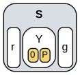
It has a site r that binds the receptor, a tyrosine Y that is either unphosphorylated (0) or phosphorylated (P), and a site g that binds DNA (Figure 2.2). A component can have both a state and a bond. A molecule with no components, such as mSOCS(), is just a species name, as in Chapter 1.
Figure 2.2: The STAT molecule type S(r,Y~0~P,g), drawn from the model file. The molecule is gray, its components white, and the allowed states of Y yellow.
2.3 Complexes are graphs
Molecules join into complexes through bonds between components. The species LRSp from Chapter 1, a ligand-bound receptor carrying phosphorylated STAT, is written
L(r!1).R(l!1,s!2).S(r!2,Y~P,g)
The dot (.) joins molecules in the same complex. A bond is written as ! followed by a label on each of its two ends: !1 on the ligand’s r and on the receptor’s l says those two components are bound to each other. Bond labels only need to be unique within a species. A component with no !, like g here, is free.
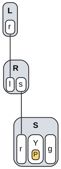
Figure 2.3: The complex L(r!1).R(l!1,s!2).S(r!2,Y~P,g). Each molecule contains its components, the yellow box gives the state of Y, and lines are bonds between components.
A species is therefore a graph (Figure 2.3). Many strings describe the same graph: molecules can be listed in any order and bonds numbered in any way. BioNetGen recognizes when two strings describe the same species by comparing their graphs.
2.4 Patterns
A pattern describes a set of species by listing only the parts that matter. The guiding principle is don’t write, don’t care: any component not mentioned in a pattern may be in any state and bound or not. Within a pattern:
a component with no bond notation must be free;
!+ means bound to any partner;
!? means bound or not;
a state such as ~P must match exactly.
A pattern matches a species if it can be found anywhere in the species’ graph. Table 2.1 shows which species from Chapter 1 match several patterns.
Table 2.1: Patterns and the species they match.
Pattern
LR
LRS
LRSp
Sp
GSp
LR·SOCS
Meaning
S(Y~P)
\(\checkmark\)
\(\checkmark\)
\(\checkmark\)
any phosphorylated STAT
S(r,Y~P)
\(\checkmark\)
\(\checkmark\)
phosphorylated, not on a receptor
S(r!+)
\(\checkmark\)
\(\checkmark\)
STAT bound through r
R(l!+)
\(\checkmark\)
\(\checkmark\)
\(\checkmark\)
\(\checkmark\)
ligand-bound receptor
R(l!+,s)
\(\checkmark\)
… with its docking site free
R(s!+)
\(\checkmark\)
\(\checkmark\)
\(\checkmark\)
docking site occupied
Observables are patterns
Observables are defined by patterns, which solves the bookkeeping problem we met in Chapter 1. There, total pSTAT had to be defined by listing every species that contains it:
Molecules pSTAT LRSp Sp GSp
With structured molecules we describe the property instead:
Molecules pSTAT S(Y~P)
The pattern continues to match every pSTAT-containing species as new complexes are added to the model, so the observable never needs to be rewritten.
A Molecules observable counts every match of its pattern, so a STAT dimer with two phosphotyrosines contributes 2 to S(Y~P), whereas a Species observable counts each matching complex once. Anticipating the STAT dimers introduced later in this chapter, in which STAT gains a dimerization site d, the observable
Species pSTATdimer S(Y~P,d!1).S(Y~P,d!1)
counts complexes that contain a dimer of two phosphorylated STATs. A complex that contained two such dimers would still count once.
2.5 Rules
A reaction rule has the same form as a reaction, but its reactants and products are patterns. Here is the rule for STAT recruitment:
The reactant patterns on the left say what must be present: a ligand-bound receptor whose docking site s is free, and an unphosphorylated STAT whose site r is free.
The product pattern on the right says what changes: a bond forms between s and r.
Everything not mentioned is carried along unchanged. If the receptor were part of a larger complex, the whole complex would take part.
Each reaction generated by the rule gets the rule’s rate constant, multiplied by any statistical factor that arises from identical molecules or sites (Chapter 4), and its rate follows mass action.
The parts of a reactant pattern that are not changed by the rule, here l!+ and the state Y~0, are its context, which restricts where the rule applies. A rule can perform five kinds of operation:
Operation
Example
form a bond
A(b) + B(a) -> A(b!1).B(a!1)
break a bond
A(b!1).B(a!1) -> A(b) + B(a)
change a state
S(Y~0) -> S(Y~P)
create a molecule
G(s!+) -> G(s!+) + mSOCS()
delete a molecule
SOCS(r) -> 0
Rule diagrams
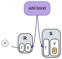
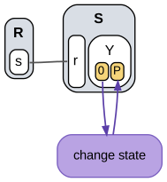
A rule can also be drawn. In a rule diagram, the reactant patterns are drawn as graphs, and each operation the rule performs is a separate node with arrows to the parts of the patterns that it changes (Sekar et al. 2017). Everything else in the diagram is context. Figure 2.4 shows the diagrams that BioNetGen generates for Sbind and for the rule that phosphorylates STAT on the receptor,
Sact: R(s!1).S(r!1,Y~0) -> R(s!1).S(r!1,Y~P) kact
(a) Sbind
(b) Sact
Figure 2.4: Rule diagrams generated from stat_rbm1_rules.bngl. Molecules are gray, components white, and internal states yellow. Purple nodes are the operations each rule performs, with arrows to the components or states they change. Gray lines and the + node are context.
Molecules are drawn as gray boxes, their components as white boxes inside them, and internal states as yellow boxes inside the components. In Sbind the operation forms a bond between the docking site s of the receptor and the site r of STAT. The rest is context. The + attached to l is a bond to an unspecified partner, written l!+ in the rule, and the yellow 0 requires unphosphorylated STAT. In Sact the operation changes the state of Y from 0 to P, and the gray line is a bond between receptor and STAT that must already exist. A component drawn without a line must be free, whereas a component that the rule does not mention, such as the site g of STAT, is not drawn at all, since it does not affect whether the rule applies. Reading a rule as a diagram thus separates the question of what a rule does from the question of where it applies.
2.6 The Chapter 1 model as rules
We now rewrite the model of Chapter 1 with structured molecules. Six molecule types replace twelve species names, and seed species list the complexes present at the start. Every other species will be generated from these by the rules.
beginmoleculetypes L(r) # ligand with one receptor-binding site R(l,s) # receptor chain: ligand site l, docking site s (shared by STAT and SOCS) S(r,Y~0~P,g) # STAT: receptor site r, tyrosine Y (unphosphorylated/phosphorylated), DNA site g G(s) # SOCS gene promoter with a STAT-binding site mSOCS() # SOCS mRNA (no internal structure) SOCS(r) # SOCS protein with a receptor-binding siteendmoleculetypesbeginseedspecies L(r) L0 R(l,s) R0 S(r,Y~0,g) S0 G(s) G0endseedspeciesbeginobservablesMolecules pSTAT S(Y~P)Molecules LRtot L(r!1).R(l!1)Molecules mSOCS mSOCS()Molecules SOCS SOCS()endobservables
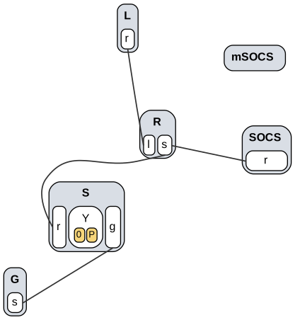
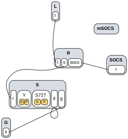
A contact map summarizes the molecule types of a model and the bonds that its rules can form (Figure 2.5). BioNetGen draws one from a model with the action visualize({type=>"contactmap"}). Each molecule type appears once, with its components and their internal states, and each line joins two components that some rule can bind. The SOCS mRNA, which has no components, appears as a box with no lines. A contact map shows which interactions are possible, but not the conditions under which they occur. For example, it shows that STAT and SOCS both bind the docking site s, but not that they bind only receptors that carry ligand. That information is the context of the rules.
Figure 2.5: Contact map of stat_rbm1_rules.bngl. Each line joins two components that a rule of the model can bind.
The receptor has a single docking site s that STAT and SOCS compete for, which is how the model of Chapter 1 treats SOCS. The rules are:
Context encodes the assumptions of the earlier model. R(l,s) in LRbind says that ligand binds and leaves only when the docking site is empty, so ligand can leave LR but not LRS. R(l!+,s) in Sbind and SOCSbind says that only ligand-bound receptors recruit STAT or SOCS.
Network generation
BioNetGen turns rules into a reaction network by network generation:
Start with the seed species.
Apply every rule to every species, or pair of species, that matches its reactant patterns.
Add any new species and reactions produced.
Repeat until nothing new appears.
The generate_network action does this and writes the result to a .net file. ODE and stochastic simulations then use the generated network. bngsim’s Model.from_bngl also generates the network, so we can check the result directly:
named = bngsim.Model.from_bngl(model_path("ch01", "stat_step6_feedback"))rules = bngsim.Model.from_bngl(model_path("ch02", "stat_rbm1_rules"))print("named species:", named.n_species, "species,", named.n_reactions, "reactions")print("rule-based: ", rules.n_species, "species,", rules.n_reactions, "reactions")for name in rules.species_names:print(" ", name)
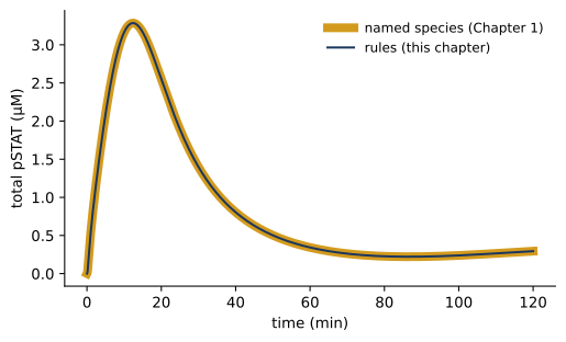
The rules generate the same 12 species and 15 reactions as the hand-written network, now with structured names. Figure 2.6 confirms that the two models give identical dynamics.
Code
for model, style, label in [(named, dict(color="#D39B1E", lw=6), "named species (Chapter 1)"), (rules, dict(color="#1B365D", lw=1.5), "rules (this chapter)")]: sim = bngsim.Simulator(model, method="ode") model.reset() r = sim.run(t_span=(0, 120), n_points=1201) plt.plot(r.time, r.observables["pSTAT"], label=label, **style)plt.xlabel("time (min)")plt.ylabel("total pSTAT (µM)")plt.legend();
Figure 2.6: The rule-based model generates the same network as the model of Chapter 1, so their predictions are identical.
2.7 Relaxing the assumptions
We now make the model more realistic by relaxing its simplifying assumptions one at a time. Each version is a separate file in models/ch02/, and each changes only a few lines.
Ligand can leave any receptor complex
Removing the context s from the ligand rule lets ligand bind and unbind whatever the receptor’s docking site is doing:
STAT docking and activation still require bound ligand, but STAT can undock from a receptor that has lost its ligand. A reversible rule applies the same context in both directions, so the binding and unbinding of STAT (and of SOCS) are now written as separate rules:
# STAT docks on a ligand-bound receptorSbind: R(l!+,s) + S(r,Y~0) -> R(l!+,s!1).S(r!1,Y~0) kSon# Unphosphorylated STAT undocksSunbind: R(s!1).S(r!1,Y~0) -> R(s) + S(r,Y~0) kSoff# Receptor-associated kinase activates docked STATSact: R(l!+,s!1).S(r!1,Y~0) -> R(l!+,s!1).S(r!1,Y~P) kact
As a result, LRbind alone now generates four binding reactions, one each for ligand binding to R alone, to R·S, to R·Sp, and to R·SOCS, together with four matching unbinding reactions, none of which had to be written by hand.
SOCS binds its own site and blocks kinase activity
In the first model SOCS blocks STAT docking by occupying the same site. SOCS proteins act differently in cells, where SOCS1 inhibits JAK directly and SOCS3 inhibits JAK while bound to the receptor. We give the receptor a separate SOCS site and require it to be free for STAT activation:
R(l,s,socs) # receptor chain: ligand site l, STAT docking site s, SOCS site socsR(l,s,socs) R0# Receptor-associated kinase activates docked STATSact: R(l!+,socs,s!1).S(r!1,Y~0) -> R(l!+,socs,s!1).S(r!1,Y~P) kact# SOCS binds a ligand-bound receptorSOCSbind: R(l!+,socs) + SOCS(r) -> R(l!+,socs!1).SOCS(r!1) kSOCSon# SOCS unbindsSOCSunbind: R(socs!1).SOCS(r!1) -> R(socs) + SOCS(r) kSOCSoff
The free socs component in Sact means that activation happens only when SOCS is absent. A receptor can now carry STAT and SOCS at the same time.
Cytokines bring two receptor chains together
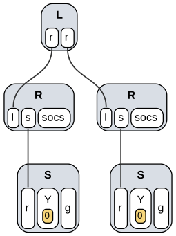
Many cytokine receptors signal when the cytokine brings together two receptor chains whose JAKs activate each other. The chains are often of different types, some receptors are assembled before the cytokine binds, and some cytokines assemble larger complexes. We take the simplest case, in which a ligand with two identical sites bridges two identical chains, and require the dimer for activation (Figure 2.7):
L(r,r) # bivalent ligand: two identical receptor-binding sitesL(r,r) L0# Ligand binds a free receptorLRbind: L(r,r) + R(l) <-> L(r!1,r).R(l!1) kon, koff# Ligand already bound to one receptor captures a second (receptor dimer)Crosslink: L(r!+,r) + R(l) <-> L(r!+,r!1).R(l!1) kx, koff# Receptor-associated kinase activates docked STATSact: L(r!+,r!2).R(l!2,socs,s!1).S(r!1,Y~0) -> L(r!+,r!2).R(l!2,socs,s!1).S(r!1,Y~P) kact
Figure 2.7: A cytokine bridging two receptor chains, each carrying an unphosphorylated STAT, one of the species generated from stat_rbm4_receptor_dimer.bngl.
BioNetGen accounts automatically for the two identical ligand sites. A free ligand can bind a receptor through either site, so the generated reaction has a statistical factor of 2. In addition, a bivalent ligand in large excess occupies receptor chains one at a time and prevents crosslinking, so the response falls at high dose. This version therefore lowers \(L_0\) from 10 to 1 µM.
STATs act as dimers
Phosphorylated STATs form dimers, and it is the dimer that binds DNA. We add a dimerization site and let free pSTAT dimerize. Only dimers bind the SOCS promoter, and only monomers are dephosphorylated:
S(r,Y~0~P,d,g) # STAT: receptor site r, tyrosine Y, dimerization site d, DNA site g# Phosphatase deactivates free monomeric pSTATSdephos: S(r,d,g,Y~P) -> S(r,d,g,Y~0) kdephos# Free pSTAT dimerizesSdimer: S(r,Y~P,d) + S(r,Y~P,d) <-> S(r,Y~P,d!1).S(r,Y~P,d!1) kdim, kundim# pSTAT binds the SOCS promoterGbind: S(d!+,g) + G(s) <-> S(d!+,g!1).G(s!1) kGon, kGoff
S(d!+,g) matches any STAT that is in a dimer and not yet on DNA. We restricted dimerization to free pSTAT because, if receptor-bound STATs could also dimerize, dimers could bridge receptor complexes into chains of any length and the network would be infinite. Network generation would never finish unless limited, for example with the max_agg option, which caps the size of complexes.
A second phosphorylation site
STAT3 is also phosphorylated on serine 727. We treat this as a separate process that does not depend on the state of tyrosine 705, an assumption that could be changed by adding Y~0 or Y~P to the context of the rule. The change requires one new component and a single rule:
S(r,Y~0~P,S727~0~P,d,g) # STAT: receptor site r, tyrosine Y, serine S727, dimerization site d, DNA site g# Ser727 is phosphorylated and dephosphorylated in any contextSser: S(S727~0) <-> S(S727~P) kser, kserdephos
The rule mentions only S727, so it applies to STAT in every complex: free, on the receptor, in a dimer, and on DNA. Every species containing one STAT now comes in two versions, and every species containing two STATs in three or four.
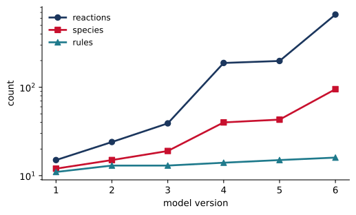
Table 2.2 counts the rules in each version and the species and reactions that BioNetGen generates from them.
Code
import pandas as pdversions = [("stat_rbm1_rules", "Chapter 1 model as rules"), ("stat_rbm2_ligand_release", "ligand leaves any complex"), ("stat_rbm3_socs_site", "separate SOCS site"), ("stat_rbm4_receptor_dimer", "receptor dimers"), ("stat_rbm5_stat_dimer", "STAT dimers"), ("stat_rbm6_ser727", "Ser727 site")]rows, models = [], {}for i, (name, change) inenumerate(versions, start=1): m = bngsim.Model.from_bngl(model_path("ch02", name)) models[i] = m rows.append({"version": i, "change": change, "rules": rule_count("ch02", name),"species": m.n_species, "reactions": m.n_reactions})sizes = pd.DataFrame(rows).set_index("version")sizes
Table 2.2: Rules in each model version and the size of the generated network.
change
rules
species
reactions
version
1
Chapter 1 model as rules
11
12
15
2
ligand leaves any complex
13
15
24
3
separate SOCS site
13
19
39
4
receptor dimers
14
40
188
5
STAT dimers
15
43
198
6
Ser727 site
16
95
663
Code
for col, marker in [("reactions", "o"), ("species", "s"), ("rules", "^")]: plt.semilogy(sizes.index, sizes[col], marker=marker, label=col)plt.xlabel("model version")plt.ylabel("count")plt.xticks(sizes.index)plt.legend();
Figure 2.8: From 11 to 16 rules, the generated network grows from 15 to 663 reactions.
Five relaxed assumptions added five rules but grew the network more than fortyfold. Writing 663 reactions and the ODEs for 95 species by hand would be slow and error-prone. Rules let us write down the mechanism and leave the bookkeeping to the software.
Figure 2.9: Contact map of stat_rbm6_ser727.bngl, the final version of the model.
The contact map grows in the same way as the rules. Figure 2.9 shows the contact map of version 6, which has 11 components and 5 possible bonds, compared with 8 and 4 in version 1 (Figure 2.5). The new components are the SOCS site on the receptor and the dimerization site and serine on STAT. The second site of the ligand adds nothing, since a contact map draws identical sites once. The loop on the site d of STAT is the bond between the two STATs of a dimer. The contact map remains small enough to read at a glance, while the network it implies does not.
2.9 Mechanistic details change the predictions
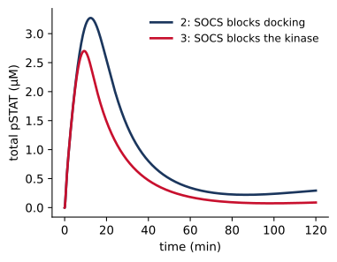
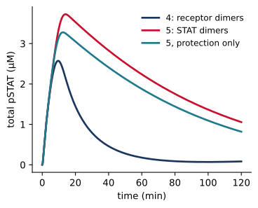
Each version embodies a different hypothesis about the mechanism, and the hypotheses make different predictions. Since the versions were built cumulatively, however, consecutive versions can differ in more than one way, and an effect can be attributed to a mechanism only by comparing models that differ in that mechanism alone. Versions 2 and 3 differ only in where SOCS binds. Versions 4 and 5 differ in two ways, since in version 5 dimerization protects pSTAT from the phosphatase and only dimers bind the SOCS promoter. To separate these, we construct a variant of version 5 in which pSTAT binds the promoter whether or not it is in a dimer, as in version 4 (Figure 2.10).
Code
import tempfile, osdef run_pSTAT(m): sim = bngsim.Simulator(m, method="ode") m.reset()return sim.run(t_span=(0, 120), n_points=1201)def half_decay(r):# time after the peak at which pSTAT first falls to half its peak value p, t = r.observables["pSTAT"], r.time i = p.argmax()return t[i + np.argmax(p[i:] < p[i] /2)]# variant of version 5: promoter binding as in version 4src = model_path("ch02", "stat_rbm5_stat_dimer").read_text()old ="Gbind: S(d!+,g) + G(s) <-> S(d!+,g!1).G(s!1)"assert old in srcwith tempfile.TemporaryDirectory() as d: path = os.path.join(d, "v5_protection_only.bngl")open(path, "w").write(src.replace(old, "Gbind: S(r,Y~P,g) + G(s) <-> S(r,Y~P,g!1).G(s!1)")) v5p = bngsim.Model.from_bngl(path, cache=False)runs = {"2: SOCS blocks docking": run_pSTAT(models[2]),"3: SOCS blocks the kinase": run_pSTAT(models[3]),"4: receptor dimers": run_pSTAT(models[4]),"5: STAT dimers": run_pSTAT(models[5]),"5, protection only": run_pSTAT(v5p)}tau = {k: half_decay(r) for k, r in runs.items()}peak = {k: r.observables["pSTAT"].max() for k, r in runs.items()}for keys in [list(runs)[:2], list(runs)[2:]]: fig, ax = plt.subplots(figsize=(4.2, 3.2))for k in keys: ax.plot(runs[k].time, runs[k].observables["pSTAT"], label=k) ax.set_xlabel("time (min)") ax.set_ylabel("total pSTAT (µM)") ax.legend() plt.show()
(a)
(b)
Figure 2.10: Controlled comparisons of mechanisms. (a) SOCS blocks STAT docking (version 2) or the kinase (version 3); the models are otherwise identical. (b) Version 4, version 5, and a variant of version 5 in which dimerization protects pSTAT from the phosphatase but monomers can still bind the SOCS promoter. All three have \(L_0\) = 1 µM.
In the first comparison, blocking the kinase (version 3) gives a lower peak, 2.70 µM rather than 3.27 µM, and a faster shutoff than blocking docking (version 2). pSTAT falls to half its peak 22 min after stimulation rather than at 27 min. Since this is the only difference between the two models, the change can be attributed to the site at which SOCS acts. In the second comparison, pSTAT falls to half its peak at 22 min without dimers and at 75 min with them. Protection from the phosphatase alone delays this time to 70 min, so it accounts for most of the longer response, and the requirement that only dimers bind the promoter accounts for the rest. These comparisons demonstrate that mechanistic details that are easy to overlook can change the predicted response substantially. Deciding which mechanism operates in cells requires experiments, and rules make it easy to build the alternative models and compare their predictions, which is the first step in designing experiments that distinguish them.
2.10 When networks are too large to generate
Network generation works well when the network is small, but realistic models can imply far more species than can be listed. A rule-based model of T cell receptor signaling with 20 molecule types and 129 rules (Chylek et al. 2014), and the ErbB model mentioned above (Creamer et al. 2012), are too large for network generation. Some models, like the STAT model with dimerization on receptors, are infinite.
Network-free simulation avoids generating the network at all. It tracks individual molecules and their bonds, and applies rules to them as the simulation runs, so only the complexes that actually form are ever represented (Sneddon et al. 2011). The cost per simulated event depends on the number of rules and molecules rather than the size of the network. The trade-offs are that network-free simulation is stochastic and works with molecule counts rather than concentrations. bngsim provides two network-free simulators, and a later chapter covers them in detail.
2.11 Summary
Multi-site proteins create combinatorial complexity, in which a few interactions imply many species and reactions.
BNGL represents molecules as objects with components, states, and bonds, so species are graphs.
Patterns specify only what matters (don’t write, don’t care), and define observables that stay correct as a model grows.
Rules transform patterns. One rule generates every reaction that fits its pattern, and context restricts where it applies.
A contact map shows which components of a model can bind, and a rule diagram shows what a rule changes and the context in which it applies. BioNetGen generates both from the model.
BioNetGen generates the network from rules for ODE and stochastic simulation. Network-free methods simulate models whose networks are too large to generate.
2.12 Exercises
In stat_rbm1_rules.bngl, change R(l,s) to R(l) in LRbind. Generate the network. Which new species appear, and why?
Write an observable for receptors that carry both STAT and SOCS in stat_rbm3_socs_site.bngl. Should it be a Molecules or a Species observable?
In stat_rbm4_receptor_dimer.bngl, vary L0 from 0.01 to 100 µM and plot the peak of total pSTAT against L0. Explain the shape of the curve.
Remove the r context from Sdimer in stat_rbm5_stat_dimer.bngl, so that receptor-bound pSTAT can dimerize. What happens when you generate the network? Try adding max_agg=>6 to generate_network.
Sketch by hand the rule diagrams for SOCSbind in stat_rbm1_rules.bngl and in stat_rbm3_socs_site.bngl. Then draw them with rule_diagram from scripts/bookutils.py, or with the action visualize({type=>"ruleviz_operation"}). Which parts of the diagrams differ, and what does the difference mean for the competition between STAT and SOCS?
2.13 Further reading
Hlavacek et al. (2006) reviews the motivation for rule-based modeling and its applications. Faeder et al. (2009) and Sekar and Faeder (2012) cover BNGL syntax and modeling practice in depth, including many examples of rules for common signaling mechanisms. Sneddon et al. (2011) introduces network-free simulation with NFsim. Sekar et al. (2017) describes the contact maps and rule diagrams that BioNetGen generates, and methods for visualizing larger models.
Blinov, Michael L., James R. Faeder, Byron Goldstein, and William S. Hlavacek. 2004. “BioNetGen: Software for Rule-Based Modeling of Signal Transduction Based on the Interactions of Molecular Domains.”Bioinformatics 20 (17): 3289–91. https://doi.org/10.1093/bioinformatics/bth378.
Chylek, Lily A., Vyacheslav Akimov, Jörn Dengjel, et al. 2014. “Phosphorylation Site Dynamics of Early T-Cell Receptor Signaling.”PLoS ONE 9 (8): e104240. https://doi.org/10.1371/journal.pone.0104240.
Creamer, Matthew S., Edward C. Stites, Meraj Aziz, et al. 2012. “Specification, Annotation, Visualization and Simulation of a Large Rule-Based Model for ERBB Receptor Signaling.”BMC Systems Biology 6: 107. https://doi.org/10.1186/1752-0509-6-107.
Faeder, James R., Michael L. Blinov, and William S. Hlavacek. 2009. “Rule-Based Modeling of Biochemical Systems with BioNetGen.”Methods in Molecular Biology 500: 113–67. https://doi.org/10.1007/978-1-59745-525-1_5.
Hlavacek, William S., James R. Faeder, Michael L. Blinov, Richard G. Posner, Michael Hucka, and Walter Fontana. 2006. “Rules for Modeling Signal-Transduction Systems.”Science’s STKE 2006 (344): re6. https://doi.org/10.1126/stke.3442006re6.
Sekar, John A. P., and James R. Faeder. 2012. “Rule-Based Modeling of Signal Transduction: A Primer.”Methods in Molecular Biology 880: 139–218. https://doi.org/10.1007/978-1-61779-833-7_9.
Sekar, John Arul Prakash, Jose-Juan Tapia, and James R. Faeder. 2017. “Automated Visualization of Rule-Based Models.”PLOS Computational Biology 13 (11): e1005857. https://doi.org/10.1371/journal.pcbi.1005857.
Sneddon, Michael W., James R. Faeder, and Thierry Emonet. 2011. “Efficient Modeling, Simulation and Coarse-Graining of Biological Complexity with NFsim.”Nature Methods 8 (2): 177–83. https://doi.org/10.1038/nmeth.1546.