Consider a receptor with distinct ligand-binding sites a and b. We can write a binding rule for each site without specifying the occupancy of the other, as in Chapter 2. If occupation of one site changes the affinity of the other, however, the corresponding rate constants must satisfy a constraint. Both orders of ligand addition reach the same doubly occupied receptor, so both must give the same equilibrium free-energy change.
Energy-based modeling expresses this constraint by assigning free energies to molecular structures and using energy differences to determine ratios of forward and reverse rate constants. Sekar, Hogg, and Faeder implemented this approach in BioNetGen (Sekar et al. 2016). We retain rules to specify which structural changes can occur; energy patterns determine how the local environment changes their rates. Thus energies become another way to parameterize the models developed in the preceding chapters.
NoteLearning goals
After this chapter you should be able to:
test whether reversible binding rates satisfy detailed balance;
construct energy patterns for binding and cooperative interactions;
derive equilibrium constants and interpret the kinetic parameters of an energy-based rule;
account for symmetry when comparing generated rates with equilibrium measurements;
distinguish equilibrium constraints from the constraints on a chemically driven signaling model;
choose energy and kinetic parameters for estimation from data.
8.1 A steady state with a circulating flux
Denote the receptor states by \(R_{00}\), \(R_{10}\), \(R_{01}\), and \(R_{11}\), where the subscripts give the occupancy of a and b. Addition of ligand follows either path around the square:
Each forward step consumes a free ligand molecule, which is omitted from the diagram. Let \(K_{A0}=k^+_{A0}/k^-_{A0}\) be the association constant for site a when b is empty, and define the other constants similarly. Detailed balance means that the forward and reverse fluxes of each elementary reversible reaction are equal at equilibrium. Applying that condition along both paths gives
The ligand concentration cancels when we compare the paths. We therefore require \(K_{A0}K_{B1}/(K_{B0}K_{A1})=1\) for passive binding, whatever the total amounts of receptor and ligand.
Consider the following context-dependent rules. The parameter boost increases association at b when a is occupied, while all other rates retain their original values.
The cycle ratio is boost. The rules still conserve receptor and ligand, and an ODE simulation still approaches a steady state. To test equilibrium we must examine reaction fluxes as well as concentrations:
bad = load("two_site_inconsistent")bad_result = run(bad)o = bad_result.observableskon, koff, boost = (bad.get_param(p) for p in ("kon", "koff", "boost"))currents = {"A binds first": kon*o["Lfree"]*o["R00"] - koff*o["R10"],"B binds second": boost*kon*o["Lfree"]*o["R10"] - koff*o["R11"],"A leaves": koff*o["R11"] - kon*o["Lfree"]*o["R01"],"B leaves": koff*o["R01"] - kon*o["Lfree"]*o["R00"],}bad_current =float(currents["A binds first"][-1])print("Final clockwise fluxes (uM/min):")for name, current in currents.items():print(f"{name:18s}{current[-1]:.6g}")
Final clockwise fluxes (uM/min):
A binds first      0.0115861
B binds second     0.0115861
A leaves           0.0115861
B leaves           0.0115861
The final currents agree at approximately 0.0116 \(\mu\)M/min. Receptor enters and leaves each state at equal rates, which explains the constant concentrations, but ligand addition and removal continue to circulate around the cycle. The binding model contains no fuel or other driving process to sustain that current. The parameter choice therefore fails a thermodynamic test even though it passes conservation and steady-state tests.
Given an explicit chemical driving process, a circulating current could be physical. We return to that case in Section 8.5. For the present binding model, the cycle constraint determines how a change in affinity at one site must be accompanied by a change at the other.
8.2 Free energies of molecular structures
Write \(g=G/(RT)\) for a dimensionless free energy, where \(R\) is the gas constant and \(T\) is the absolute temperature. For our receptor, assign binding contributions \(g_A\) and \(g_B\), and an additional contribution \(g_{AB}\) when both sites are occupied:
The free-energy change on binding at a is \(g_A\) when b is empty and \(g_A+g_{AB}\) when b is occupied. Binding at b gives \(g_B\) or \(g_B+g_{AB}\). Both routes to \(R_{11}\) therefore sum to the same energy.
An energy pattern assigns a free-energy contribution to each occurrence of a specified molecular structure. BioNetGen sums the contributions of all matching patterns to obtain the energy of a species. The patterns for the receptor are:
beginenergypatterns R(a!1).L(r!1) gA R(b!1).L(r!1) gB R(a!+,b!+) gABendenergypatterns
The first pattern counts an a–ligand bond, the second counts a b–ligand bond, and the third counts a receptor with both sites bound. The third pattern need not name the ligand molecules since their identities are already restricted by the binding rules. In a model where several kinds of partner can bind those sites, the pattern would need additional context if the cooperative energy were specific to one partner.
Receptor structure
Matching contributions
Relative energy
R(a,b)
none
\(0\)
R(a!1,b).L(r!1)
a bond
\(g_A\)
R(a,b!1).L(r!1)
b bond
\(g_B\)
R(a!1,b!2).L(r!1).L(r!2)
both bonds and double occupancy
\(g_A+g_B+g_{AB}\)
Concentration references and affinity
For association of two distinct molecules, use a concentration reference \(C_{\mathrm{ref}}\) to form a dimensionless equilibrium constant. If the dissociation constant is \(K_D\), then
A more negative binding energy corresponds to a smaller dissociation constant. The numerical value of the energy depends on the concentration reference. A conventional thermodynamic standard state and a computational reference expressed in micromolar units require a corresponding conversion of the association energy; the predicted physical affinity must agree.
Our BNGL models use micromolar concentrations, minutes, and \(C_{\mathrm{ref}}=1\ \mu\)M. The parameter Cref records that convention; BioNetGen’s Arrhenius expression uses the numerical rates in those units and does not read Cref as a separate unit conversion. Keep Cref fixed when running these files. Changing concentration units requires converting the bimolecular rates and association energies together.
beginparameters R0 1 L0 1 Cref 1# concentration reference (uM); keep at 1 here KD_A 0.1# isolated-site dissociation constant (uM) KD_B 0.1 omega 10# enhancement of affinity when the other site binds gA ln(KD_A/Cref) gB ln(KD_B/Cref) gAB -ln(omega) kA 1# kinetic scale (1/min) kB 1 EA -ln(kA) # log kinetic scale relative to 1/min EB -ln(kB) phi 0# allocation of energy change to forward rateendparameters
Here \(g_{AB}=-\ln\omega\), where \(\omega\) is the factor by which occupation of one site increases the affinity of the other. Given \(\omega>1\), the doubly occupied receptor receives a favorable energy contribution. Thus \(K_{D,A\mid B}=K_{D,A}/\omega\) and \(K_{D,B\mid A}=K_{D,B}/\omega\). The same cooperative factor applies in both directions, as required by the cycle constraint. An unfavorable interaction has \(\omega<1\).
These are effective free energies of the molecular states represented in the model. Solvent effects and unresolved conformations can contribute to them. An energy pattern therefore need not correspond to a bond energy calculated from an atomic structure, and its parameter can be estimated from affinity measurements.
8.3 From energy differences to rates
Equilibrium constrains a ratio of rates. To predict a time course we also need a kinetic scale. BioNetGen supplies the reversible rate law Arrhenius(phi,Ea), which computes numerical forward and reverse rates from the dimensionless energy change \(\Delta g\):
Their ratio is \(e^{-\Delta g}\). The parameter \(E_a\) determines their common scale, while \(\phi\) determines how an energy change is divided between the forward and reverse rates. We usually restrict \(\phi\) to the interval from zero to one in this phenomenological parameterization.
For the association convention used here, write the dimensional rates as
The BNGL parameter EA = -ln(kA) sets the numerical kinetic scale relative to the time reference in the file. Taking a logarithm of a rate requires that reference; EA is an effective parameter rather than a measured activation energy. In our concentration convention, the numerical association rate produced by Arrhenius has units of \(\mu\)M\(^{-1}\)min\(^{-1}\) and the dissociation rate has units of min\(^{-1}\).
Each rule leaves the other receptor site unspecified. BioNetGen generates the relevant reactions, evaluates their energy differences, and gives them the corresponding rates. At \(\phi=0\), the association rate is independent of context, while the dissociation rate changes with affinity. At \(\phi=1\), the dissociation rate is independent of context. Intermediate values change both rates. None of these choices changes the equilibrium constant.
Checking the generated dynamics
We can express the same model with ordinary mass-action rules by specifying the occupancy of the other site and deriving each rate explicitly:
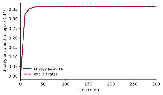
The file two_site_rates.bngl defines the rates using the equations above. For example, konAB and koffAB use \(\Delta g=g_A+g_{AB}\). Comparing the generated time courses checks that the energy rules give the intended kinetics, including the context-dependent dissociation rates.
energy = load("two_site_energy")explicit = load("two_site_rates")energy_result = run(energy)explicit_result = run(explicit)max_difference =max( np.max(np.abs(energy_result.observables[n] - explicit_result.observables[n]))for n in energy.observable_names)plt.plot(energy_result.time, energy_result.observables["R11"], label="energy patterns")plt.plot(explicit_result.time, explicit_result.observables["R11"],"--", label="explicit rates")plt.xlabel("time (min)")plt.ylabel("doubly occupied receptor (µM)")plt.xlim(0, 300)plt.legend()plt.show()
Figure 8.1: Doubly occupied receptor in the energy-based and explicit-rate models. Both start with free receptor and free ligand.
The maximum absolute difference across the observables is 2.2e-14 \(\mu\)M for this calculation. At the final state, every reversible reaction also balances individually:
e = energy_result.observableska = energy.get_param("kA")ga, gab = energy.get_param("gA"), energy.get_param("gAB")first_flux = ka*e["Lfree"][-1]*e["R00"][-1] - ka*np.exp(ga)*e["R10"][-1]second_flux = ka*e["Lfree"][-1]*e["R01"][-1] - ka*np.exp(ga+gab)*e["R11"][-1]print(f"A binding, B empty: {first_flux:.3g} uM/min")print(f"A binding, B occupied: {second_flux:.3g} uM/min")
A binding, B empty:    8.86e-16 uM/min
A binding, B occupied: -1.07e-15 uM/min
The calculation uses the default \(\phi=0\); the identical site parameters give the same balance at b. The numerical residuals reflect integration tolerance. Energy-based parameterization has removed the circulating flux of Section 8.1 by enforcing the relation between both binding paths.
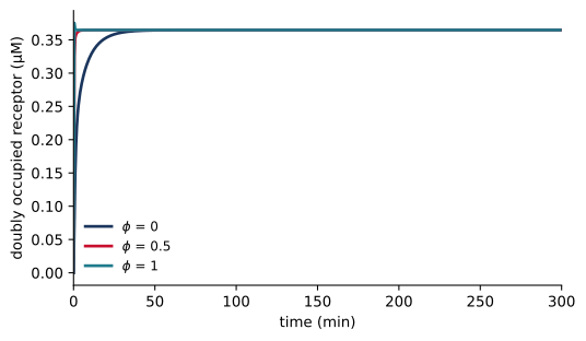
for phi in (0, 0.5, 1): r = run(energy, end=300, n_points=601, phi=phi) plt.plot(r.time, r.observables["R11"], label=f"$\\phi$ = {phi:g}")plt.xlim(0, 300)plt.xlabel("time (min)")plt.ylabel("doubly occupied receptor (µM)")plt.legend()plt.show()energy.set_param("phi", 0)
Figure 8.2: Changing the allocation parameter changes relaxation while preserving the equilibrium occupancy.
Since binding is favorable in this example, increasing \(\phi\) increases both rates at fixed \(E_a\). The receptor therefore approaches the same equilibrium more rapidly (Figure 8.2). An affinity measurement alone cannot determine which allocation gives the observed relaxation.
8.4 Cooperativity and a binding polynomial
At a specified free ligand concentration, define \(x_A=[L]/K_{D,A}\) and \(x_B=[L]/K_{D,B}\). The equilibrium weights of the receptor states are \(1\), \(x_A\), \(x_B\), and \(\omega x_Ax_B\). Their sum is the binding polynomial
\[
Z=1+x_A+x_B+\omega x_Ax_B.
\]
Dividing each weight by \(Z\) gives its receptor fraction. In particular, \(f_{11}=\omega x_Ax_B/Z\). These fractions use free ligand concentration. In a closed experiment the measured input is often total ligand, so we must also impose
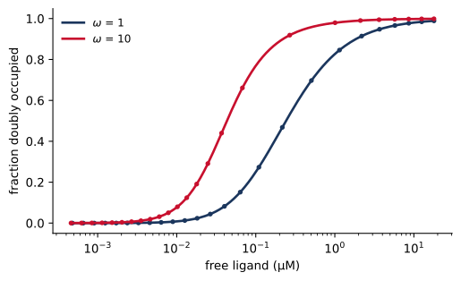
Figure 8.3: Equilibrium double occupancy with independent sites and favorable coupling. Lines are binding-polynomial predictions evaluated at the simulated free ligand concentration; points are ODE results.
Favorable coupling moves double occupancy toward lower free ligand concentrations. The largest difference between the simulated and predicted fractions is 1.6e-08. Using total ligand in \(x_A\) and \(x_B\) would violate the mass balance when receptor binding depletes the free pool.
A reciprocal interaction between RAF dimerization and drug binding
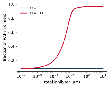
Poulikakos and coworkers observed that RAF inhibitors can increase ERK signaling in cells with wild-type BRAF, and connected this response to RAF dimers (Poulikakos et al. 2010). Consider an illustrative assembly model in which inhibitor binding favors RAF dimerization. We represent each RAF protomer by a dimerization site d and an inhibitor site i.
The first pattern assigns an energy to a dimer bond and the second to an inhibitor bond. The third assigns a coupling contribution to each inhibitor-bound protomer in a dimer. It has one match in a singly occupied dimer and two in a doubly occupied dimer. Thus binding an inhibitor stabilizes the dimer, and dimerization increases inhibitor affinity by the same coupling factor. The reciprocal effect follows from the shared energy assignment.
The dimer bond joins identical molecules. BioNetGen counts that symmetric energy pattern once per bond and includes a factor of one half in the generated association rate for two identical free protomers. With the present parameter convention, the macroscopic dissociation constant of the inhibitor-free dimer is therefore
The parameter KD_dim defines \(C_{\mathrm{ref}}e^{g_{\mathrm{Dim}}}\) in this file; the measured macroscopic constant includes the additional symmetry factor. Association of inhibitor to an empty dimer has a factor of two because either protomer can bind, while inhibitor dissociation from a doubly occupied dimer has the corresponding factor of two. Generated statistical factors must be included when comparing rate constants with a bulk equilibrium constant.
To explore the consequence of the coupling, suppose that an unoccupied protomer in a dimer is catalytically available, a drug-bound protomer is inhibited, and a monomer contributes no activity. The observable Active counts available protomers under those assumptions. It is an activity proxy; the model contains no substrate turnover or downstream ERK reactions, and its parameters are illustrative.
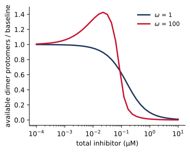
Figure 8.4: An illustrative RAF assembly model, without coupling (\(\omega\) = 1) and with favorable coupling (\(\omega\) = 100). (a) Available dimer protomers relative to their number without inhibitor. Favorable coupling increases this number at low inhibitor concentrations, and inhibitor occupancy reduces it at higher doses. (b) Fraction of RAF in dimers.
With favorable coupling, the available-protomer count reaches 1.43 times its inhibitor-free value in this scan. At low doses, inhibitor recruits RAF into dimers, creating additional unoccupied dimer partners. As the dose rises, occupation of those partners reduces the activity proxy even though the dimer fraction remains high. Removing the coupling gives the comparison curve in Figure 8.4. The calculation demonstrates a possible assembly mechanism for a nonmonotonic response; predicting a cellular ERK response would require additional catalytic reactions and experimental constraints.
8.5 Equilibrium and chemically driven signaling
A signaling pathway can maintain currents by consuming chemical fuel. For example, a kinase and a phosphatase can carry a substrate around the cycle
where \(a_i\) is a dimensionless activity. With ATP, ADP, and phosphate maintained by external processes, their chemical potentials can sustain \(\Delta G_{\mathrm{hyd}}<0\). Such externally maintained pools are called chemostats. The substrate concentrations can then become stationary while phosphorylation and dephosphorylation continue at equal nonzero rates.
Local detailed balance relates the forward-to-reverse propensity ratio of an elementary transition to its free-energy change, including changes in the reservoirs. Around the complete fuel-consuming cycle, the dimensionless forward-to-reverse product is \(\exp[-\Delta G_{\mathrm{hyd}}/(RT)]\). A favorable hydrolysis reaction therefore permits a product different from unity. For a closed system at equilibrium, the chemical potentials adjust until the net affinity of each cycle vanishes.
Assigning energies only to \(S\) and \(S_P\) and applying the same reversible energy law to both enzyme channels would eliminate this driving force. A driven model must represent the fuel reaction explicitly or retain its chemical-potential contribution in effective forward and reverse rates. For an enzymatic mechanism, this constraint applies to elementary steps; a fitted irreversible rate or a coarse-grained catalytic rate can describe a regime where the reverse flux is negligible, but it does not by itself specify the complete thermodynamic cycle.
Garcia and coworkers used thermodynamic constraints in a model of mitochondrial ATP production (Garcia et al. 2023). Energy-based binding and assembly modules can likewise be combined with driven catalytic modules in a signaling model, provided that the reservoir contributions and reaction conventions are consistent. A global demand that every signaling reaction balance individually would remove the sustained activity that the model is intended to describe.
8.6 Choosing parameters for calibration
For the two-site receptor, the equilibrium parameters are \(g_A\), \(g_B\), and \(g_{AB}\), or equivalently \(K_{D,A}\), \(K_{D,B}\), and \(\omega\). Given those parameters, the four context-dependent affinity constants are constrained. There are three independent equilibrium parameters, since the cycle constraint removes one degree of freedom from the four affinity constants. The kinetic scales for the two binding rules and their allocation parameters determine how the system approaches equilibrium.
An equilibrium binding curve can constrain affinity and coupling, provided that the measurements distinguish their effects. It contains no direct information about the kinetic scale. Conversely, association and washout time courses can constrain rates, particularly when experiments probe several ligand concentrations and occupancy contexts. At a single fixed energy difference, different combinations of \(E_a\) and \(\phi\) can give the same forward and reverse rates, so estimating both requires additional context or an imposed kinetic assumption.
In the RAF example, an activity-proxy curve combines dimer formation with inhibitor occupancy. Measurements of the dimer fraction and bound inhibitor would constrain these processes more directly. Since activity also depends on our assumption about which protomers can signal, fitting a curve cannot establish that assumption without independent evidence.
Energy parameters can be shared across many reactions generated by a rule. Such sharing reduces the number of independent affinity parameters and enforces cycle consistency, but the chosen patterns still express a mechanistic hypothesis. If coupling depends on a third component or a conformation omitted from the pattern, a fit may compensate by shifting the available energy parameters. The parameter-estimation and uncertainty chapters develop ways to distinguish a well-constrained energy from a parameter that absorbs missing model structure.
8.7 Summary
In a passive binding model, the product of association constants around any cycle of reactions must be the same in both directions. A model that violates this condition can still conserve mass and reach a steady state, but its steady state carries a circulating flux that no energy source sustains.
An energy pattern assigns a free-energy contribution to each occurrence of a molecular structure, and BioNetGen sums the contributions to obtain the energy of each species. Cooperative effects defined this way are reciprocal, and every cycle is consistent.
The Arrhenius rate law sets the ratio of forward and reverse rates from the energy change. Ea sets their common scale and phi divides the energy change between them, and neither affects the equilibrium.
The binding polynomial gives equilibrium occupancies as functions of the free ligand concentration. In a closed system the free concentration follows from mass balance.
Statistical factors for identical molecules and sites enter the generated rates and must be included when rate constants are compared with measured equilibrium constants.
A signaling pathway driven by ATP hydrolysis maintains currents that a closed system at equilibrium cannot. A driven model must represent the fuel or its chemical potential rather than impose detailed balance on every reaction.
Equilibrium measurements constrain energies, while time courses are needed to constrain the kinetic parameters.
8.8 Exercises
Derive the cycle constraint for the two-site receptor directly from the four equilibrium mass-action equations. In two_site_inconsistent.bngl, change a second rate so that the cycle ratio becomes unity. Confirm conservation and individual reaction balance after simulation.
Set KD_A and KD_B to different values in two_site_energy.bngl. Derive all four equilibrium weights and compare the binding-polynomial prediction with the ODE result. Explain why cooperative enhancement must remain reciprocal even for unequal sites.
Compare independent, favorable, and unfavorable coupling. Plot double occupancy against both total and free ligand. Identify the regime in which ligand depletion changes the interpretation of the input dose.
At fixed affinities, change the kinetic scales and phi. Design association and dissociation measurements that could discriminate among the resulting time courses. State which parameters would remain ambiguous if only equilibrium occupancy were measured.
Inspect the network generated from raf_inhibitor_energy.bngl. Identify the symmetry factors in dimer association and inhibitor binding. Derive the inhibitor-free dimer equilibrium and verify it numerically at several total RAF concentrations.
Replace the RAF activity proxy by the concentration of entirely inhibitor-free dimers. Compare its dose response with the proxy in Figure 8.4 and explain which mechanistic assumption changed.
Write effective forward and reverse rate ratios for the kinase and phosphatase cycle that include the nucleotide and phosphate activities. Show that their product is determined by the ATP-hydrolysis free energy. Explain how a stationary substrate distribution can coexist with continuing fuel consumption.
8.9 Further reading
Sekar, Hogg, and Faeder describe energy patterns and their implementation in BioNetGen (Sekar et al. 2016). The accompanying models in this chapter provide small tests of cycle consistency, rate allocation, and symmetry. Poulikakos and coworkers provide the experimental RAF example (Poulikakos et al. 2010), while Garcia and coworkers illustrate thermodynamic constraints in ATP production (Garcia et al. 2023).
Garcia, Guadalupe C., Kavya Gupta, Thomas M. Bartol, Terrence J. Sejnowski, and Padmini Rangamani. 2023. “Mitochondrial Morphology Governs ATP Production Rate.”Journal of General Physiology 155 (9): e202213263. https://doi.org/10.1085/jgp.202213263.
Poulikakos, Poulikos I., Chao Zhang, Gideon Bollag, Kevan M. Shokat, and Neal Rosen. 2010. “RAF Inhibitors Transactivate RAF Dimers and ERK Signalling in Cells with Wild-Type BRAF.”Nature 464 (7287): 427–30. https://doi.org/10.1038/nature08902.
Sekar, John A. P., Justin S. Hogg, and James R. Faeder. 2016. “Energy-Based Modeling in BioNetGen.”2016 IEEE International Conference on Bioinformatics and Biomedicine (BIBM), 1460–67. https://doi.org/10.1109/BIBM.2016.7822739.