3  Stochastic simulation and noise

The differential equations of Chapter 1 treat the amount of each species as a continuous quantity that changes smoothly and predictably in time. This is a good description when every species is present in large numbers. A cell, however, typically contains one or two copies of a given gene, a few to a few hundred copies of each mRNA, and proteins in numbers ranging from tens to millions. At the low end of this range, the timing of individual reaction events matters, and genetically identical cells exposed to the same signal respond differently. In this chapter we describe a reaction network by the numbers of molecules it contains and by the probabilities of the reactions that change them, simulate it with the stochastic simulation algorithm, and use the simulations to ask how random fluctuations shape the response of the cytokine–STAT–SOCS circuit.

NoteLearning goals

After this chapter you should be able to:

• convert a model written in concentrations into one written in molecule numbers;
• explain what a reaction propensity is and how it is related to a rate constant;
• describe Gillespie’s stochastic simulation algorithm and implement it for a simple reaction;
• explain how the size of fluctuations depends on the number of molecules;
• describe how bursts of transcription arise and how they propagate through a feedback loop;
• run stochastic simulations with bngsim and analyze ensembles of trajectories.

3.1 Why molecule numbers matter

The idea that biochemical noise can be measured, rather than merely supposed, was established by experiments in single cells. In 2002 Elowitz and coworkers placed two copies of the same promoter, driving two fluorescent proteins of different colors, into the same Escherichia coli cells (Elowitz et al. 2002). If expression were deterministic, each cell would contain equal amounts of the two proteins. Instead, the cells varied in two ways. The total amount of the two proteins differed from cell to cell, with the two colors rising and falling together, and within a single cell the two colors differed from each other. Elowitz and coworkers called the correlated part of the variation extrinsic noise, since it arises from differences among cells in factors that affect both genes, such as the amounts of polymerase and ribosomes. They called the uncorrelated part intrinsic noise, since it arises from the random timing of transcription and translation of each gene, and they found that both make substantial contributions to the variation among cells. Since then, cell-to-cell variation in gene expression has been found in organisms from bacteria to mammals, with consequences for stress responses, development, and cell fate decisions (Raj and Oudenaarden 2008).

Consider the SOCS gene in our model. In Chapter 1 the promoter G had a concentration of 1 µM, which in a cell of 1 pL volume corresponds to about 600,000 copies. The real number is one or two. A single promoter is either bound by pSTAT or not, and it produces mRNA only while it is bound, so the production of SOCS mRNA is a sequence of discrete events whose timing is random. The question we want to answer is whether this randomness matters for the signaling response, and if so, which features of the response it affects.

3.2 From concentrations to molecule numbers

To describe a network by molecule numbers we need the number of molecules that corresponds to a given concentration. For a volume \(V\) in liters, 1 µM corresponds to

\[ N_AV \times 10^{-6}\ \text{molecules per µM}, \]

where \(N_A = 6.022\times10^{23}\) mol⁻¹ is Avogadro’s number. In a 1 pL mammalian cell this is about \(6\times10^5\) molecules per µM, so 1 nM corresponds to about 600 molecules. In a bacterium of 1 fL volume, 1 nM corresponds to less than one molecule.

Rate constants must be converted as well. A first-order rate constant, with units of inverse time, is unchanged, since it describes what happens to each molecule independently. A second-order rate constant in µM⁻¹ min⁻¹ is divided by the number of molecules per µM to give a constant per pair of molecules. In BNGL we carry out these conversions in the parameters block, so that the model can still be written in terms of familiar concentrations. Here is the ligand–receptor model of Chapter 1 written this way:

begin parameters
  NAV      100               # molecules per uM in the reaction volume
  L0_uM    1                 # ligand (uM)
  R0_uM    1                 # receptor (uM)
  kon_uM   1                 # binding (1/uM/min)
  koff     0.1               # unbinding (1/min)
  L0       rint(L0_uM*NAV)   # ligand (molecules)
  R0       rint(R0_uM*NAV)   # receptor (molecules)
  kon      kon_uM/NAV        # binding (1/molecule/min)
end parameters

The parameter NAV is the number of molecules per µM. With NAV = 100 the model contains 100 ligand and 100 receptor molecules, which corresponds to a reaction volume of about 0.17 fL. BioNetGen does not perform these conversions automatically for models without compartments. It treats the numbers in the species block as amounts in whatever units the rate constants assume, and it is up to the modeler to keep the two consistent. A later chapter on compartments shows how BioNetGen can handle volumes explicitly.

3.3 The stochastic description of a reaction network

In the stochastic description, the state of the system at time \(t\) is the vector \(\mathbf{x}\) of molecule numbers, and each reaction \(j\) has a propensity \(a_j(\mathbf{x})\), defined so that \(a_j(\mathbf{x})\,dt\) is the probability that one reaction event of type \(j\) occurs in the next small time interval \(dt\). For an elementary reaction the propensity is the per-molecule rate constant multiplied by the number of distinct combinations of reactant molecules. For ligand–receptor binding and unbinding,

\[ a_1 = k_\mathrm{on}\,x_\mathrm{L}\,x_\mathrm{R}, \qquad a_2 = k_\mathrm{off}\,x_\mathrm{LR}, \]

where \(k_\mathrm{on}\) is now the per-molecule constant. For a reaction between two molecules of the same type, the number of distinct pairs is \(x(x-1)/2\), and BioNetGen accounts for the corresponding symmetry factors when it generates the network.

The probability \(P(\mathbf{x},t)\) of finding the system in state \(\mathbf{x}\) obeys the chemical master equation,

\[ \frac{dP(\mathbf{x},t)}{dt} = \sum_j \left[\, a_j(\mathbf{x}-\boldsymbol{\nu}_j)\,P(\mathbf{x}-\boldsymbol{\nu}_j,t) - a_j(\mathbf{x})\,P(\mathbf{x},t)\,\right], \tag{3.1}\]

where \(\boldsymbol{\nu}_j\) is the column of the stoichiometry matrix for reaction \(j\), the change in \(\mathbf{x}\) when reaction \(j\) fires. The first term in the brackets is the flux of probability into state \(\mathbf{x}\) from the states that lead to it, and the second is the flux out. Equation 3.1 is a system of linear equations with one equation for every possible state. For all but the smallest networks the number of states is far too large to solve it directly, so instead we sample trajectories of the process it describes. When the volume and the numbers of all molecules grow together, the fluctuations become small compared with the mean, and the trajectories approach the solution of the ODEs of Chapter 1. At finite numbers, the mean of the stochastic process obeys the ODEs only for networks of first-order reactions. For a bimolecular reaction the mean rate depends on the average of a product, such as \(\langle L R \rangle\), which differs from the product of the averages, \(\langle L \rangle \langle R \rangle\), whenever the two numbers fluctuate together. The difference is small when the numbers are large, but it need not be small in general.

3.4 Gillespie’s algorithm

In 1977 Daniel Gillespie described a method for generating trajectories that are exact samples of the process described by Equation 3.1. The method, now called the stochastic simulation algorithm (SSA) or Gillespie’s algorithm, follows directly from the definition of the propensity. Since the probability that each reaction fires in the next short interval depends only on the current state, the waiting time until the next event of any kind is exponentially distributed with rate \(a_0 = \sum_j a_j(\mathbf{x})\), and the probability that the next event is reaction \(j\) is \(a_j/a_0\). One step of the algorithm is thus:

1. Compute the propensities \(a_j(\mathbf{x})\) and their sum \(a_0\).
2. Draw a random number \(r_1\) uniformly from \((0,1)\) and advance time by \(\tau = -\ln(r_1)/a_0\).
3. Draw a second random number \(r_2\) and choose reaction \(j\) with probability \(a_j/a_0\).
4. Update the state, \(\mathbf{x} \leftarrow \mathbf{x} + \boldsymbol{\nu}_j\), and repeat.

The algorithm is short enough to write ourselves for ligand–receptor binding:

rng = np.random.default_rng(1)

def gillespie(L, R, LR, kon, koff, t_end):
    """Exact stochastic simulation of L + R <-> LR."""
    t, times, counts = 0.0, [0.0], [LR]
    while True:
        a1, a2 = kon * L * R, koff * LR          # propensities
        a0 = a1 + a2
        if a0 == 0:                              # no reaction can occur
            break
        t += -np.log(rng.random()) / a0          # time to the next event
        if t > t_end:                            # next event is too late
            break
        if rng.random() * a0 < a1:               # choose which event
            L, R, LR = L - 1, R - 1, LR + 1
        else:
            L, R, LR = L + 1, R + 1, LR - 1
        times.append(t)
        counts.append(LR)
    times.append(t_end)                          # hold the last state to t_end
    counts.append(LR)
    return np.array(times), np.array(counts)

t_hand, LR_hand = gillespie(L=100, R=100, LR=0, kon=0.01, koff=0.1, t_end=20)

In bngsim the same simulation is a change of method. The model file defines the conversion to molecule numbers, so nothing else needs to change. Figure 3.1 compares one trajectory from each implementation with the ODE solution.

model = bngsim.Model.from_bngl(model_path("ch03", "lr_counts"))
ssa = bngsim.Simulator(model, method="ssa")
ode = bngsim.Simulator(model, method="ode")

model.reset()
r_ssa = ssa.run(t_span=(0, 20), n_points=201, seed=2)
model.reset()
r_ode = ode.run(t_span=(0, 20), n_points=201)

plt.step(t_hand, LR_hand, where="post", lw=1, label="SSA, Python implementation")
plt.step(r_ssa.time, r_ssa.observables["LR"], where="post", lw=1, label="SSA, bngsim")
plt.plot(r_ode.time, r_ode.observables["LR"], "k--", lw=1.5, label="ODE")
plt.xlabel("time (min)")
plt.ylabel("LR (molecules)")
plt.legend(loc="lower right");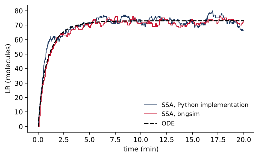

Figure 3.1: Stochastic simulations of ligand–receptor binding with 100 ligand and 100 receptor molecules, from the Python implementation above and from bngsim, compared with the ODE solution. Both trajectories fluctuate about the deterministic curve. The Python implementation records every event, so its trajectory moves in steps of one molecule. bngsim records the state at 201 evenly spaced times, so a single step in its trajectory can contain several events.

Every stochastic simulation with a different random seed gives a different trajectory. The seed argument makes a run reproducible, and run_replicates runs many trajectories with seeds seed, seed + 1, and so on, which is how we build up the statistics in the rest of this chapter.

3.5 Noise and system size

Consider the same binding reaction in volumes of different size, with the concentrations and rate constants held fixed. The ODE solution is identical in every case, since it depends only on concentrations, but the stochastic trajectories are not. Figure 3.2 shows that the relative size of the fluctuations shrinks as the number of molecules grows.

fig, ax = plt.subplots(figsize=(4.2, 3.2))
for NAV in [10, 100, 1000]:
    model.set_param("NAV", NAV)
    model.reset()
    r = ssa.run(t_span=(0, 20), n_points=401, seed=4)
    ax.plot(r.time, r.observables["LR"] / NAV, lw=1, label=f"NAV = {NAV}")
model.set_param("NAV", 100)
model.reset()
ax.plot(r_ode.time, r_ode.observables["LR"] / 100, "k--", lw=1.5)
ax.set_xlabel("time (min)")
ax.set_ylabel("[LR] (µM)")
ax.legend(loc="lower right")
plt.show()

navs = np.array([10, 30, 100, 300, 1000, 3000])
mean_lr, cv_lr = [], []
for NAV in navs:
    model.set_param("NAV", NAV)
    model.reset()
    reps = ssa.run_replicates(400, t_span=(0, 30), n_points=31, seed=5)
    x = np.array([rep.observables["LR"][-1] for rep in reps])
    mean_lr.append(x.mean())
    cv_lr.append(x.std() / x.mean())
model.set_param("NAV", 100)
mean_lr, cv_lr = np.array(mean_lr), np.array(cv_lr)

fig, ax = plt.subplots(figsize=(4.2, 3.2))
ax.loglog(mean_lr, cv_lr, "o-")
ax.loglog(mean_lr, cv_lr[0] * np.sqrt(mean_lr[0] / mean_lr), "k--", lw=1)
ax.set_xlabel("mean number of LR complexes")
ax.set_ylabel("coefficient of variation")
plt.show()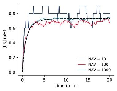

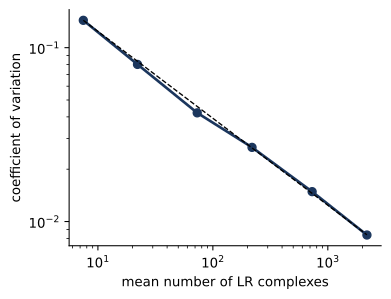
(a)

(b)

Figure 3.2: Fluctuations shrink as the number of molecules grows. (a) Single trajectories of [LR] at three values of NAV, the number of molecules per µM, with the ODE solution (dashed). (b) Coefficient of variation of the number of complexes at equilibrium, from 400 trajectories at each volume. The dashed line has slope −1/2.

With about 7 complexes at equilibrium, the standard deviation of the number of complexes is 14% of the mean. With about 2189 complexes it is 0.8%. The coefficient of variation falls as \(1/\sqrt{N}\), the dependence expected when a quantity is the sum of many independent random events. This scaling explains why the ODEs work well for species that are abundant and whose fluctuations arise from their own reactions. For a Poisson distribution, the coefficient of variation is \(1/\sqrt{\langle N \rangle}\), so a protein present at 10,000 copies would fluctuate by 1%, which is smaller than the precision of most of the measurements we want to explain. More generally, the square of the coefficient of variation is the Fano factor, defined in the next section, divided by the mean. Processes that produce molecules in bursts, or that inherit fluctuations from a species present at small numbers, have large Fano factors, and an abundant protein made from a single gene can fluctuate far more than the Poisson value. Noise thus matters most in species present at small numbers and in the processes they drive.

3.6 Bursts in gene expression

Gene expression is the clearest example of a process driven by small numbers. Figure 3.3 shows the simplest model that captures it, in which a promoter switches between an inactive and an active state, and mRNA is made only while the promoter is active (Peccoud and Ycart 1995). The model uses a structured molecule, Gene(p~off~on), whose component p records the state of the promoter.

begin parameters
  kact     0.05    # promoter activation (1/min)
  kinact   0.05    # promoter inactivation (1/min)
  ktx      4       # transcription from the active promoter (1/min)
  kdeg     0.1     # mRNA degradation (1/min)
end parameters

begin molecule types
  Gene(p~off~on)
  mRNA()
end molecule types

begin seed species
  Gene(p~off)  1
end seed species

begin observables
  Molecules GeneOn  Gene(p~on)
  Molecules mRNA    mRNA()
end observables

begin reaction rules
  Switch:     Gene(p~off) <-> Gene(p~on)        kact, kinact
  Transcribe: Gene(p~on) -> Gene(p~on) + mRNA()  ktx
  Degrade:    mRNA() -> 0                       kdeg
end reaction rules

At steady state, the mean number of mRNA molecules is the rate of transcription from the active promoter, multiplied by the fraction of time the promoter is active, divided by the rate constant for degradation:

\[ \langle m \rangle = \frac{k_\mathrm{tx}}{k_\mathrm{deg}}\, \frac{k_\mathrm{act}}{k_\mathrm{act} + k_\mathrm{inact}}, \]

which is 20 for the parameters above. The mean says nothing about how expression is distributed in time, however. A useful measure of noise is the Fano factor, the variance divided by the mean, which equals 1 for a Poisson distribution. For this model with a single promoter, at steady state,

\[ \frac{\sigma_m^2}{\langle m \rangle} = 1 + \frac{k_\mathrm{tx}\,k_\mathrm{inact}} {(k_\mathrm{act} + k_\mathrm{inact})(k_\mathrm{act} + k_\mathrm{inact} + k_\mathrm{deg})}. \tag{3.2}\]

When the promoter switches rapidly compared with mRNA degradation, the second term becomes small, and the distribution of mRNA approaches the Poisson distribution that transcription at a constant rate would give. When the promoter switches slowly compared with mRNA degradation, and many transcripts are made in each period of activity, each period produces a burst of transcripts, and the distribution becomes much broader. Figure 3.3 compares the two cases, which have the same mean.

gene = bngsim.Model.from_bngl(model_path("ch03", "gene_expression"))
gssa = bngsim.Simulator(gene, method="ssa")
cases = {"slow switching": 0.05, "fast switching": 50}

fig, ax = plt.subplots(figsize=(4.2, 3.2))
for label, k in cases.items():
    gene.set_param("kact", k)
    gene.set_param("kinact", k)
    gene.reset()
    r = gssa.run(t_span=(0, 500), n_points=1001, seed=8)
    ax.step(r.time, r.observables["mRNA"], where="post", lw=1, label=label)
ax.set_xlabel("time (min)")
ax.set_ylabel("mRNA (molecules)")
ax.legend(loc="upper left")
plt.show()

fano = {}
fig, ax = plt.subplots(figsize=(4.2, 3.2))
for label, k in cases.items():
    gene.set_param("kact", k)
    gene.set_param("kinact", k)
    gene.reset()
    reps = gssa.run_replicates(2000, t_span=(0, 200), n_points=3, seed=7)
    m = np.array([rep.observables["mRNA"][-1] for rep in reps])
    fano[label] = m.var() / m.mean()
    if label == "slow switching":
        zero_frac = np.mean(m == 0)
        high_frac = np.mean(m > 2 * m.mean())
    ax.hist(m, bins=np.arange(0, 80, 2), alpha=0.6, density=True, label=label)
ax.set_xlabel("mRNA (molecules)")
ax.set_ylabel("probability per molecule")
ax.legend()
plt.show()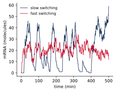

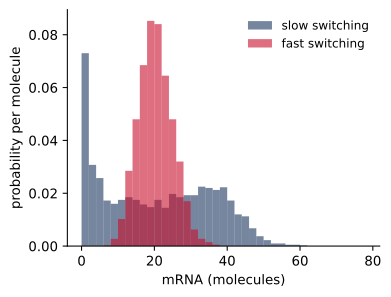
(a)

(b)

Figure 3.3: Transcriptional bursting. Slow promoter switching (\(k_\mathrm{act} = k_\mathrm{inact} = 0.05\) min⁻¹) and fast switching (50 min⁻¹) give the same mean of 20 mRNA molecules but very different fluctuations. (a) Single trajectories. (b) Distributions of mRNA number across 2000 cells at \(t\) = 200 min.

The simulated Fano factors are 11.2 for slow switching and 1.09 for fast switching, compared with 11.0 and 1.02 from Equation 3.2. With slow switching, 10% of cells contain no mRNA at all at a given moment, while 9% contain more than twice the mean. A protein made from these transcripts averages over the bursts for a time set by its own lifetime, so bursting matters most when the protein is short-lived or when its effect depends on how much is present at a particular moment.

3.7 A noisy feedback loop

We now return to the cytokine–STAT–SOCS circuit and give it a single copy of the SOCS gene. The model stat_ssa_feedback.bngl is the rule-based model of Chapter 2 written in molecule numbers. To keep the simulations fast, it uses NAV = 1000, so that the receptor is present at 1000 copies, STAT at 10,000, and the gene at one. A real mammalian cell has a volume about 1000 times larger, with correspondingly more copies of the abundant proteins, but the same one or two copies of the gene. The gene-expression rate constants are chosen so that the fully induced gene gives about 20 SOCS mRNA molecules.

NAV       1000             # molecules per uM in the reaction volume
G0        1                # SOCS gene copies
kGon      1/NAV            # pSTAT-promoter binding (1/molecule/min)
kGoff     1                # pSTAT-promoter unbinding (1/min)
ktx       2.5              # transcription from the bound promoter (1/min)
ktl       12               # translation (1/min)

Figure 3.4 shows ten individual cells, the mean of 200 cells, and the ODE solution of the same model.

stat = bngsim.Model.from_bngl(model_path("ch03", "stat_ssa_feedback"))
sssa = bngsim.Simulator(stat, method="ssa")
sode = bngsim.Simulator(stat, method="ode")

stat.reset()
cells = sssa.run_replicates(200, t_span=(0, 240), n_points=481, seed=11)
P = np.array([c.observables["pSTAT"] for c in cells])
t = cells[0].time
stat.reset()
r_det = sode.run(t_span=(0, 240), n_points=481)

fig, ax = plt.subplots(figsize=(4.2, 3.2))
for p in P[:10]:
    ax.plot(t, p, color="0.6", lw=0.8)
ax.plot(t, P.mean(axis=0), color="#1B365D", lw=2, label="mean of 200 cells")
ax.plot(r_det.time, r_det.observables["pSTAT"], "k--", lw=1.5, label="ODE")
ax.set_xlim(0, 120)
ax.set_xlabel("time (min)")
ax.set_ylabel("total pSTAT (molecules)")
ax.legend()
plt.show()

peak_cv = P.max(axis=1).std() / P.max(axis=1).mean()
late = P[:, -1]
late_cv = late.std() / late.mean()

stat.set_param("kGoff", 0.05)          # slower switching, same occupancy
stat.set_param("kGon", 0.05 / 1000)
stat.reset()
slow = sssa.run_replicates(200, t_span=(0, 240), n_points=481, seed=11)
late_slow = np.array([c.observables["pSTAT"][-1] for c in slow])
late_slow_cv = late_slow.std() / late_slow.mean()
stat.set_param("kGoff", 1)
stat.set_param("kGon", 1 / 1000)

fig, ax = plt.subplots(figsize=(4.2, 3.2))
bins = np.linspace(0, 1600, 33)
ax.hist(late, bins=bins, alpha=0.6, density=True, label="default switching")
ax.hist(late_slow, bins=bins, alpha=0.6, density=True, label="slow switching")
ax.set_xlabel("adapted pSTAT (molecules)")
ax.set_ylabel("probability per molecule")
ax.legend()
plt.show()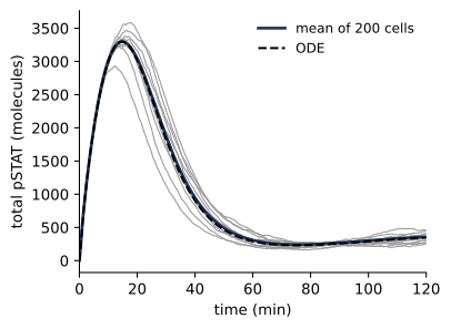

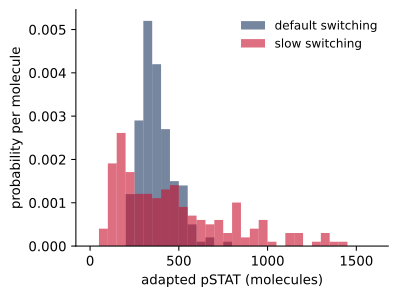
(a)

(b)

Figure 3.4: Stochastic simulation of the cytokine–STAT–SOCS circuit with a single SOCS gene. (a) Total pSTAT in ten individual cells (gray), the mean of 200 cells (blue), and the ODE solution (dashed). (b) Distribution of the adapted pSTAT level at 240 min across 200 cells, for the default parameters and for a promoter that switches 20 times more slowly with the same occupancy.

The mean of many cells follows the ODE solution closely, and the peak is nearly the same in every cell: its coefficient of variation is 5%. This is because the peak occurs before the feedback acts. It is set by the binding and activation reactions, which involve thousands of molecules, and by the time SOCS has been made the peak has passed. The adapted level, in contrast, is set by the balance between STAT activation and inhibition by SOCS, and the amount of SOCS depends on the activity of a single gene and on a handful of mRNA molecules. The adapted level thus varies by 25% from cell to cell with the default parameters, and by 69% when the promoter switches slowly.

These results show that the same circuit can make some features of its response reliable and others variable. A measurement that averages over a population, such as a western blot, reports the mean, which for this model follows the ODE solution closely. A measurement in single cells, such as flow cytometry or imaging, would reveal the spread in the adapted response, and the width of that spread carries information about the kinetics of the SOCS promoter that the population average does not.

3.8 Faster approximate methods

The cost of an exact stochastic simulation is proportional to the number of reaction events, which grows with the number of molecules. Models that contain both rare species, like a gene, and abundant ones, like a cytoplasmic protein present at millions of copies, spend nearly all of their time simulating reactions of the abundant species, whose fluctuations are small. Several approximate methods address this problem. In tau leaping each step advances time by an interval \(\tau\), chosen so that the propensities change little during it, and fires a Poisson-distributed number of each reaction (Gillespie 2007). In the partial scaling algorithm (PSA) of Lin, Feng, and Hlavacek, populations above a critical size are simulated as if they were scaled down, which reduces the number of events while leaving small populations exact (Lin et al. 2019). bngsim provides PSA through the same interface as SSA:

psa = bngsim.Simulator(model, method="psa", poplevel=100)

where poplevel is the critical population size. Larger values give more accurate results and less acceleration. Since PSA is approximate, it is good practice to compare it with exact SSA on a smaller version of the problem before relying on it. A third approach, network-free stochastic simulation, avoids generating the reaction network at all and is the subject of a later chapter.

3.9 Summary

• When species are present in small numbers, the random timing of reactions causes cells to differ, and the stochastic description is needed.
• Converting a model to molecule numbers leaves first-order rate constants unchanged and divides second-order constants by the number of molecules per µM.
• The propensity \(a_j\) of a reaction is the probability per unit time that it fires. The chemical master equation describes how the probability of each state evolves, and Gillespie’s algorithm generates exact sample trajectories.
• When all molecule numbers grow with the volume, relative fluctuations scale as \(1/\sqrt{N}\), and the ODEs describe the system well. Noise matters most for species present at small numbers and for the processes they drive, which can include abundant proteins made from a single gene.
• Slow promoter switching produces bursts of transcription, which increase the Fano factor of mRNA well above the Poisson value of 1.
• In the cytokine–STAT–SOCS circuit with a single SOCS gene, the peak of the response is nearly the same in every cell, while the adapted level varies with the activity of the gene.

3.10 Exercises

1. Implement the algorithm. Extend the gillespie function to simulate stat_step4_release.bngl from Chapter 1 in molecule numbers. Compare the mean of 100 trajectories with bngsim’s SSA and with the ODEs.
2. System size. In lr_counts.bngl, plot the full distribution of the number of LR complexes at equilibrium for NAV = 10 and 1000. How does its shape change? Why is the coefficient of variation in Figure 3.2 smaller than \(1/\sqrt{\langle N \rangle}\)?
3. Bursts. In gene_expression.bngl, keep the mean mRNA number at 20 and vary the switching rates over four orders of magnitude, with \(k_\mathrm{act} = k_\mathrm{inact}\). Plot the simulated Fano factor against the prediction of Equation 3.2.
4. Gene copy number. Give the cell in stat_ssa_feedback.bngl two copies of the SOCS gene (G0 = 2) and halve ktx, so that the mean transcription rate is unchanged. How does the spread of the adapted level change, and why?
5. Speed and accuracy. Set NAV to 30,000 in stat_ssa_feedback.bngl and compare the run time and the distribution of peak pSTAT from SSA and from PSA with poplevel = 100 and 1000.

3.11 Further reading

Gillespie (2007) reviews the theory of stochastic chemical kinetics and the exact and approximate simulation methods built on it. Raj and Oudenaarden (2008) reviews the sources and consequences of noise in gene expression, and Elowitz et al. (2002) is the experiment that separated intrinsic from extrinsic noise. Lin et al. (2019) describes the partial scaling algorithm implemented in BioNetGen and bngsim.

Elowitz, Michael B., Arnold J. Levine, Eric D. Siggia, and Peter S. Swain. 2002. “Stochastic Gene Expression in a Single Cell.” Science 297 (5584): 1183–86. https://doi.org/10.1126/science.1070919.

Gillespie, Daniel T. 2007. “Stochastic Simulation of Chemical Kinetics.” Annual Review of Physical Chemistry 58: 35–55. https://doi.org/10.1146/annurev.physchem.58.032806.104637.

Lin, Yen Ting, Song Feng, and William S. Hlavacek. 2019. “Scaling Methods for Accelerating Kinetic Monte Carlo Simulations of Chemical Reaction Networks.” The Journal of Chemical Physics 150 (24): 244101. https://doi.org/10.1063/1.5096774.

Peccoud, Jean, and Bernard Ycart. 1995. “Markovian Modeling of Gene-Product Synthesis.” Theoretical Population Biology 48 (2): 222–34. https://doi.org/10.1006/tpbi.1995.1027.

Raj, Arjun, and Alexander van Oudenaarden. 2008. “Nature, Nurture, or Chance: Stochastic Gene Expression and Its Consequences.” Cell 135 (2): 216–26. https://doi.org/10.1016/j.cell.2008.09.050.