5  Compartments and transport

The models of Part I treat the cell as a single well-mixed volume. A real cell is divided by membranes into compartments, and where a molecule is matters as much as what state it is in. A cytokine binds its receptor in the extracellular medium, the receptor sits in the plasma membrane, STAT is phosphorylated in the cytoplasm, and the SOCS gene is transcribed in the nucleus. Moving between these places takes time, and the same reaction runs at different rates in compartments of different size, since the same number of molecules gives a higher concentration in a smaller volume. In this chapter we describe the compartments of a cell in BNGL, write rules that apply in every compartment with the correct rates, write rules for transport across membranes, and use them to place the cytokine–STAT–SOCS circuit in a cell with a nucleus and endosomes.

Before compartments were part of the language, modelers encoded location as an internal state of each molecule, writing for example R(loc~surf~endo), and wrote every reaction once for each location with its own rate constant. This works, but the geometry appears nowhere in the model, the software cannot check that molecules in different places do not react, and the number of rules grows with the number of compartments. Leonard Harris, Justin Hogg, and the author introduced compartmental BNGL, or cBNGL, to address these problems (Harris et al. 2009). In cBNGL location is a property of the compartment that holds a molecule, compartments are declared with their sizes and topology, and BioNetGen scales the rate of each reaction by the size of the compartment in which it occurs.

NoteLearning goals

After this chapter you should be able to:

• declare the compartments of a cell and the topology that connects them;
• specify the location of molecules and complexes in seed species, observables, and rules;
• explain how BioNetGen scales bimolecular rate constants by compartment size, and choose units that make the scaling transparent;
• write rules for transport of molecules and complexes between compartments, including endocytosis;
• recognize the ways a compartmental model can generate reactions the modeler did not intend.

5.1 Declaring compartments

A cell is a set of nested compartments of two kinds: volumes, which are three-dimensional, and surfaces, which are the two-dimensional membranes that separate volumes. Figure 5.1 shows the compartments used in this chapter. The plasma membrane (PM) separates the extracellular medium (EC) from the cytoplasm (CP); the nuclear envelope (NM) separates the cytoplasm from the nucleus (NU); and the endosomal membrane (EM) separates the cytoplasm from the endosome lumen (EN). The tree on the right is the form BioNetGen uses. Volumes and surfaces must alternate along every branch, a surface may enclose only one volume, and a volume may contain several surfaces, as the cytoplasm contains both the nuclear and the endosomal membranes.

Figure 5.1: The compartments of a cell and their topology. Left, a cell with a nucleus and endosomes; the endosomes are lumped into one compartment in the models. Right, the tree of compartments declared in BNGL, with the dimension of each.

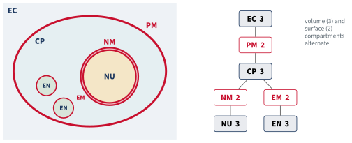
Compartments are declared in a block of their own. Each line gives a name, the dimension (3 for a volume, 2 for a surface), the size, and the compartment that encloses it. The compartments of stat_compartments.bngl are:

begin compartments
  EC  3  V_EC*NA_pL                   # extracellular medium
  PM  2  A_PM*h*um3*NA_pL     EC      # plasma membrane
  CP  3  V_CP*NA_pL           PM      # cytoplasm
  NM  2  A_NM*h*um3*NA_pL     CP      # nuclear envelope
  NU  3  V_NU*NA_pL           NM      # nucleus
end compartments

The outermost compartment, here the medium, has no parent. The size of a volume is its volume. The size of a surface is its area multiplied by an effective thickness, \(h\), which converts the area into a volume for the purpose of rate scaling, as discussed below. The value of \(h\) cancels from every comparison between surface reactions, but every surface in a model must use the same value.

5.2 Where molecules are

The location of a molecule is written with @ after it, and the location of a whole species with @ and a double colon before it. The seed species of the STAT model place each molecule in its compartment:

begin seed species
  L(r,r)@EC          L0
  R(l,s,socs)@PM     R0
  S(r,Y~0,d,g)@CP    S0
  G(s)@NU            G0
end seed species

A complex can span compartments. When the cytokine binds the receptor, the cytokine stays in the medium and the receptor stays in the membrane, and BioNetGen writes the complex as

@PM::L(r!1,r)@EC.R(l!1,s,socs)

The prefix @PM:: gives the location of the complex as a whole, and the suffix @EC gives the location of the cytokine within it. A complex is located on a surface if any of its molecules is on that surface, and in a volume only if all of its molecules are in that volume. A complex may include one surface and molecules in the two volumes adjacent to it, but no more, so a receptor in the plasma membrane can bind a ligand outside the cell and STAT inside it, but a single complex cannot reach from the plasma membrane to the nucleus.

Observables and rules may name a compartment or leave it out. The observable S()@NU counts STAT molecules in the nucleus, while S() would count STAT everywhere. A rule that names no compartment is universal, meaning that it applies to matching molecules in every compartment where they can meet, and BioNetGen works out where that is.

5.3 How compartment size sets the rate

Consider a binding reaction that occurs in both the cytoplasm and the nucleus, with the same number of molecules of A and B in each, and with the nucleus four times smaller than the cytoplasm. The model two_volumes.bngl contains one universal rule for this reaction,

# One rule, no compartment named: it applies wherever A and B meet
Bind:  A(b) + B(a) <-> A(b!1).B(a!1)   kon, koff

and BioNetGen generates one forward reaction for each compartment:

@CP::A(b) + @CP::B(a) -> @CP::A(b!1).B(a!1)  kon/(V_CP*NA_pL)  [Bind]
@NU::A(b) + @NU::B(a) -> @NU::A(b!1).B(a!1)  kon/(V_NU*NA_pL)  [Bind]
@CP::A(b!1).B(a!1) -> @CP::A(b) + @CP::B(a)  koff  [Bind, reverse]
@NU::A(b!1).B(a!1) -> @NU::A(b) + @NU::B(a)  koff  [Bind, reverse]

The rate constant of each bimolecular reaction is the rate constant of the rule divided by the size of the compartment, while the unimolecular reverse reactions are not scaled. In general, a bimolecular rate constant is divided by the size of the compartment in which the reaction occurs, and if the reactants are in a volume and on an adjacent surface, by the size of the volume. Reactions of a single reactant, including transport, are never scaled.

The scaling is simplest to follow when compartment sizes are given in units that convert concentrations to numbers of molecules. In this chapter every size is written as NAV, the number of molecules per µM in the compartment, \(N_A V \times 10^{-6}\) with \(V\) in liters (Chapter 3), which is 6.02e+05 for a volume of 1 pL. The amounts of all species are then numbers of molecules per cell, and the rate constants of the rules keep the familiar units of µM⁻¹ min⁻¹. Dividing \(k_\mathrm{on}\) by NAV gives the rate constant per pair of molecules, which is the conversion we made by hand in Chapter 3, and compartments give each part of the cell its own value of NAV.

model = bngsim.Model.from_bngl(model_path("ch05", "two_volumes"))
sim = bngsim.Simulator(model, method="ode")
model.reset()
r = sim.run(t_span=(0, 5), n_points=201)
N0 = model.get_param("N0")

fig, ax = plt.subplots(figsize=(4.2, 3.2))
ax.plot(r.time, r.observables["AB_CP"], label="cytoplasm")
ax.plot(r.time, r.observables["AB_NU"], label="nucleus")
ax.set_xlabel("time (min)")
ax.set_ylabel("AB complexes (molecules)")
ax.legend(loc="lower right")
plt.show()

fig, ax = plt.subplots(figsize=(4.2, 3.2))
ax.plot(r.time, r.observables["AB_CP"] / N0, label="cytoplasm")
ax.plot(r.time, r.observables["AB_NU"] / N0, label="nucleus")
ax.set_xlabel("time (min)")
ax.set_ylabel("fraction of A bound")
plt.show()
frac_cp = r.observables["AB_CP"][-1] / N0
frac_nu = r.observables["AB_NU"][-1] / N0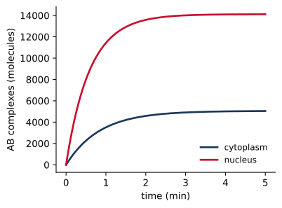

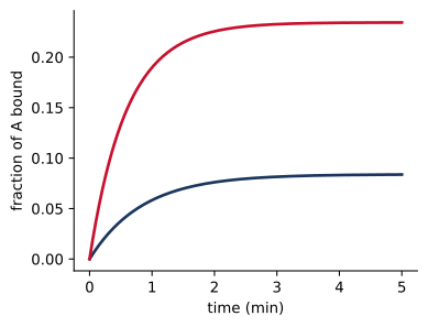
(a)

(b)

Figure 5.2: The same binding rule in two compartments. The cytoplasm (1 pL) and the nucleus (0.25 pL) start with the same numbers of A and B. (a) Number of AB complexes. (b) Fraction of A bound. Binding is faster and more complete in the nucleus, where the same numbers of molecules are four times more concentrated.

Figure 5.2 shows the consequence. With 60,220 molecules of A and of B in each compartment, the concentration of each is 0.1 µM in the cytoplasm and 0.4 µM in the nucleus. At equilibrium 8% of A is bound in the cytoplasm and 23% in the nucleus, as the dissociation constant of 1 µM predicts for these concentrations. Since the rule is written once with an intrinsic rate constant, the difference between the compartments comes entirely from their sizes. If the nucleus were made larger, the model would change only in the compartments block.

Surfaces follow the same arithmetic. Two receptors that meet in the plasma membrane react at a rate divided by the size of the membrane, which is NAV computed for an effective volume \(Ah\), the area \(A\) times an effective thickness \(h\). A smaller membrane, such as that of an endosome, concentrates its receptors and speeds their reactions in the same way. The thickness is a modeling convention rather than the physical width of a bilayer. It relates a two-dimensional rate constant \(k_\mathrm{2D}\), with units of area per molecule per time, to the three-dimensional constant used in the rule by \(k_\mathrm{3D} = k_\mathrm{2D}\,h\), so that the rate per unit area is the same in either description. We fix \(h\) at 10 nm in this chapter. If \(h\) is changed, every rate constant of a reaction in a membrane must be changed in proportion, or the two-dimensional rates the model represents will change.

It is important to note that the rate constant of a compartmental rule is an intrinsic constant, independent of compartment size. A rate constant taken from a model that wrote one rule per location, or fitted separately to each location, may have the compartment size built into it already, for example if the source model counted molecules rather than concentrations. Copying such a constant into a compartmental rule applies the scaling twice, and the model runs without complaint but with every such rate wrong by a factor of the compartment size. The scaling applies to every bimolecular rule, whether it names a compartment or not, so the equations and units of the source model should be checked before any constant is copied.

5.4 Transport

Molecules move between compartments by transport rules, which change the location of a molecule or a complex without changing its bonds or states. Transport is unimolecular, so its rate constant is not scaled. The STAT model uses three kinds:

# pSTAT dimers are imported as a unit (species transport)
Import:     @CP:S(d!1).S(d!1) -> @NU:S(d!1).S(d!1)            kimp
# unphosphorylated monomers shuttle in both directions (molecule transport)
Shuttle:    S(r,Y~0,d,g)@CP <-> S(r,Y~0,d,g)@NU               kimp0, kexp
mExport:    mSOCS()@NU -> mSOCS()@CP                          kmexp

Shuttle and mExport are molecule transport. The named molecule changes compartment, here between the cytoplasm and the nucleus across the nuclear envelope. A molecule may move between two volumes that share a surface, or between a volume and an adjacent surface, and BioNetGen rejects a move that would leave a bond spanning compartments that are not adjacent.

Import is species transport, written with the location prefix on both sides. The whole complex, here a pSTAT dimer, moves to the nucleus as a unit. The rate of species transport applies once per complex. A dimer is imported at rate kimp, the same as a complex containing only one matching molecule would be. A third form, species transport between surfaces, describes endocytosis and is taken up in Section 5.6. Finally, the keyword MoveConnected after a molecule transport rule makes the molecule carry with it the molecules bound to it in the same compartment, which is useful for cargo carried by a transport receptor (Harris et al. 2009).

5.5 STAT in a cell with a nucleus

STAT proteins carry the cytokine signal from the membrane to the nucleus. In unstimulated cells STAT1 and STAT3 shuttle between the cytoplasm and the nucleus, with most of the protein in the cytoplasm at steady state. Phosphorylated STAT dimers are imported actively and accumulate in the nucleus, where they are dephosphorylated by the nuclear phosphatase TC45 and exported again (Reich and Liu 2006; Hoeve et al. 2002). stat_compartments.bngl adds these steps to the model of Chapter 2 (version 5, with STAT dimers). The membrane and receptor rules are unchanged and name no compartment:

# --- at the membrane: no compartments named, BNG finds where each applies ---
LRbind:     L(r,r) + R(l) <-> L(r!1,r).R(l!1)                 kon, koff
Sbind:      R(l!+,s) + S(r,Y~0) -> R(l!+,s!1).S(r!1,Y~0)      kSon
# --- dimerization occurs in both cytoplasm and nucleus ---
Sdimer:     S(r,Y~P,d,g) + S(r,Y~P,d,g) <-> S(r,Y~P,d!1,g).S(r,Y~P,d!1,g)   kdim, kundim

BioNetGen places each reaction where its reactants can meet. The cytokine binds the receptor at a rate scaled by the volume of the medium, and STAT docks on the receptor at a rate scaled by the volume of the cytoplasm. pSTAT dimerizes both in the cytoplasm and in the nucleus, each at its own rate. Steps that happen in only one place name the compartment:

# --- in the nucleus ---
Sdephos:    S(d,g,Y~P)@NU -> S(d,g,Y~0)@NU                    kdephos
Transcribe: G(s!+) -> G(s!+) + mSOCS()@NU                     ktx
# --- in the cytoplasm ---
Translate:  mSOCS()@CP -> mSOCS()@CP + SOCS(r)@CP             ktl

Dephosphorylation occurs only in the nucleus, as TC45 does. Transcription produces mRNA in the nucleus, which is exported to the cytoplasm and translated there. The generated network shows the reactions that involve nuclear transport, dimerization, and the promoter:

@CP::S(Y~0,d,g,r) -> @NU::S(Y~0,d,g,r)  kimp0  [Shuttle]
@NU::S(Y~0,d,g,r) -> @CP::S(Y~0,d,g,r)  kexp  [Shuttle, reverse]
@CP::S(Y~P,d,g,r) + @CP::S(Y~P,d,g,r) -> @CP::S(Y~P,d!1,g,r).S(Y~P,d!1,g,r)  0.5*kdim/(V_CP*NA_pL)  [Sdimer]
@CP::S(Y~P,d!1,g,r).S(Y~P,d!1,g,r) -> @CP::S(Y~P,d,g,r) + @CP::S(Y~P,d,g,r)  kundim  [Sdimer, reverse]
@CP::S(Y~P,d!1,g,r).S(Y~P,d!1,g,r) -> @NU::S(Y~P,d!1,g,r).S(Y~P,d!1,g,r)  kimp  [Import]
@NU::S(Y~P,d!1,g,r).S(Y~P,d!1,g,r) -> @NU::S(Y~P,d,g,r) + @NU::S(Y~P,d,g,r)  kundim  [Sdimer, reverse]
@NU::G(s) + @NU::S(Y~P,d!1,g,r).S(Y~P,d!1,g,r) -> @NU::G(s!1).S(Y~P,d!2,g!1,r).S(Y~P,d!2,g,r)  2*kGon/(V_NU*NA_pL)  [Gbind]
@NU::S(Y~P,d,g,r) + @NU::S(Y~P,d,g,r) -> @NU::S(Y~P,d!1,g,r).S(Y~P,d!1,g,r)  0.5*kdim/(V_NU*NA_pL)  [Sdimer]
@NU::G(s!1).S(Y~P,d!2,g!1,r).S(Y~P,d!2,g,r) -> @NU::G(s) + @NU::S(Y~P,d!1,g,r).S(Y~P,d!1,g,r)  kGoff  [Gbind, reverse]

Dimerization is four times faster per pair of molecules in the nucleus than in the cytoplasm. A pSTAT dimer binds the promoter at twice the written rate, since either of its two DNA-binding sites can bind.

model = bngsim.Model.from_bngl(model_path("ch05", "stat_compartments"))
sim = bngsim.Simulator(model, method="ode")
model.reset()
r = sim.run(t_span=(0, 240), n_points=481)
o = r.observables

fig, ax = plt.subplots(figsize=(4.2, 3.2))
ax.plot(r.time, o["pSTAT_CP"])
ax.plot(r.time, o["pSTAT_NU"])
ax.set_xlabel("time (min)")
ax.set_ylabel("pSTAT (molecules)")
ax2 = ax.twinx()
ax2.plot(r.time, o["R_SOCS"], color="#5B6770", ls="--", lw=1.5)
ax2.set_ylabel("SOCS-bound receptors", color="#5B6770")
ax2.spines["right"].set_visible(True)
ax2.set_ylim(0, 1.15 * model.get_param("R0"))
ax.text(60, 12400, "nucleus", color="#C8102E", fontsize=9)
ax.text(22, 3000, "cytoplasm", color="#1B365D", fontsize=9)
ax2.text(240, 0.88 * model.get_param("R0"), "SOCS-bound\nreceptors", color="#5B6770", fontsize=9, ha="right", va="top")
plt.show()

nuc = o["STAT_NU"] / (o["STAT_NU"] + o["STAT_CP"])
# block export at 60 min: continue from the state at 60 min with kexp = 0
model.reset()
r1 = sim.run(t_span=(0, 60), n_points=121)
model.set_param("kexp", 0)
r2 = sim.run(t_span=(60, 240), n_points=361)
model.set_param("kexp", 0.2)
nuc_lmb = np.concatenate([r1.observables["STAT_NU"] / (r1.observables["STAT_NU"] + r1.observables["STAT_CP"]),
                          r2.observables["STAT_NU"] / (r2.observables["STAT_NU"] + r2.observables["STAT_CP"])])
t_lmb = np.concatenate([r1.time, r2.time])

fig, ax = plt.subplots(figsize=(4.2, 3.2))
ax.plot(r.time, nuc, label="default")
ax.plot(t_lmb, nuc_lmb, "--", label="export blocked at 60 min")
ax.set_xlabel("time (min)")
ax.set_ylabel("nuclear fraction of STAT")
ax.set_ylim(0, 1)
ax.legend(loc="upper left")
plt.show()

ptot = o["pSTAT_CP"] + o["pSTAT_NU"]
i_pk = np.argmax(ptot)
t_pk, nu_share = r.time[i_pk], o["pSTAT_NU"][i_pk] / ptot[i_pk]
nuc_pk = nuc.max()
nuc_rest = model.get_param("kimp0") / (model.get_param("kimp0") + model.get_param("kexp"))
conc_ratio = (o["pSTAT_NU"][i_pk] / model.get_param("V_NU")) / (o["pSTAT_CP"][i_pk] / model.get_param("V_CP"))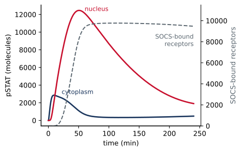

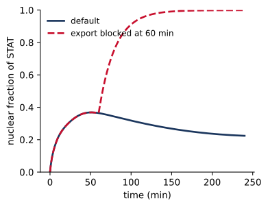
(a)

(b)

Figure 5.3: Nuclear accumulation of STAT after cytokine stimulation. (a) pSTAT molecules in the cytoplasm and the nucleus, with SOCS bound to receptors (right axis). (b) Fraction of all STAT that is in the nucleus, for the default model and with nuclear export blocked at 60 min.

Figure 5.3 shows the response to 1 nM cytokine. Total pSTAT peaks at 46 min, and at the peak 90% of it is in the nucleus. Since the nucleus is four times smaller than the cytoplasm, the concentration of pSTAT in the nucleus is then 36 times its concentration in the cytoplasm, and an image of the cell would show a bright nucleus. pSTAT accumulates in the nucleus because import of the dimer is fast and only unphosphorylated STAT is exported, so pSTAT is trapped until it is dephosphorylated. As SOCS protein accumulates and blocks the receptors, phosphorylation declines, and the nuclear fraction of STAT falls from 37% toward its resting value of 20%, which is set by the shuttling rate constants, \(k_\mathrm{imp0}/(k_\mathrm{imp0} + k_\mathrm{exp})\).

The model reproduces a classic experiment. Begitt and coworkers treated cells with leptomycin B, an inhibitor of nuclear export, after stimulation with interferon-γ and found that STAT1 remained in the nucleus instead of returning to the cytoplasm (Begitt et al. 2000). Setting kexp to zero at 60 min has the same effect in the model (Figure 5.3 b). Dephosphorylated STAT can no longer leave, and the nuclear fraction rises even as the signal declines.

5.6 Endocytosis and receptor trafficking

Many receptors are internalized after they bind ligand. The membrane around the receptor buds into the cell to form an endosome, carrying the receptor into the endosomal membrane and its bound ligand into the endosome lumen. In the acidic endosome many ligands dissociate, and free receptors are recycled to the surface while the ligand is degraded. These processes control how many receptors a cell displays and how long it responds (Lauffenburger and Linderman 1993). internalization.bngl describes them with surface-to-surface species transport:

begin reaction rules
  # Binding applies on both membranes
  LRbind:      L(r,r) + R(l) <-> L(r!1,r).R(l!1)          kon, koff
  Crosslink:   L(r!+,r) + R(l) <-> L(r!+,r!1).R(l!1)      kx, koff
  # Acidic pH speeds ligand release in endosomes
  EndoRelease: R(l!1)@EM.L(r!1) -> R(l)@EM + L(r)        koff_endo
  # Surface-to-surface species transport: the whole complex moves
  Internalize: @PM:R(l!+) -> @EM:R(l!+)                  kint
  Constitutive: @PM:R(l) -> @EM:R(l)                     kint0
  Recycle:     @EM:R(l) -> @PM:R(l)                      krec
  # Free ligand is degraded in the endosome
  LigandDeg:   L(r,r)@EN -> 0                            kdegL
end reaction rules

The rule Internalize moves any complex containing a ligand-bound receptor from the plasma membrane to the endosomal membrane. Molecules in the complex that are in the medium move into the endosome lumen, following the topology of endocytosis, in which the outside of the cell becomes the inside of the endosome:

@PM::L(r!1,r)@EC.R(l!1) -> @EM::L(r!1,r)@EN.R(l!1)  kint  [Internalize]
@PM::L(r!1,r!2)@EC.R(l!1).R(l!2) -> @EM::L(r!1,r!2)@EN.R(l!1).R(l!2)  kint  [Internalize]

The binding rules name no compartment, so they apply on the endosomal membrane as well as on the surface. This is intended, since ligand does bind receptors in endosomes, but it has a consequence that is easy to overlook. The endosome lumen is small, and the rate constant for ligand binding there is divided by its size:

@EC::L(r,r) + @PM::R(l) -> @PM::L(r!1,r)@EC.R(l!1)  2*kon/(V_EC*NA_pL)  [LRbind]
@PM::L(r!1,r)@EC.R(l!1) -> @EC::L(r,r) + @PM::R(l)  koff  [LRbind, reverse]
@EM::L(r!1,r)@EN.R(l!1) -> @EM::R(l) + @EN::L(r,r)  koff  [LRbind, reverse]
@EM::R(l) + @EN::L(r,r) -> @EM::L(r!1,r)@EN.R(l!1)  2*kon/(V_EN*NA_pL)  [LRbind]

model = bngsim.Model.from_bngl(model_path("ch05", "internalization"))
sim = bngsim.Simulator(model, method="ode")
runs = {}
for ke in [1, 100, 1000, 10000]:
    model.set_param("koff_endo", ke)
    model.reset()
    runs[ke] = sim.run(t_span=(0, 120), n_points=241)
model.set_param("koff_endo", 1000)
V_EN = model.get_param("V_EN")
R0 = model.get_param("R0")

fig, ax = plt.subplots(figsize=(4.2, 3.2))
for ke, rr in runs.items():
    ax.plot(rr.time, rr.observables["R_surface"] / R0, label=f"$k_{{off,endo}}$ = {ke:g} min⁻¹")
ax.set_xlabel("time (min)")
ax.set_ylabel("fraction of receptors on surface")
ax.set_ylim(0, 1.02)
ax.legend(loc="upper right")
plt.show()

fig, ax = plt.subplots(figsize=(4.2, 3.2))
for ke, rr in runs.items():
    line, = ax.plot(rr.time, rr.observables["L_endosome"] / (V_EN * NA_pL), label=f"{ke:g}")
    ax.plot(rr.time, rr.observables["L_free_EN"] / (V_EN * NA_pL), "--", color=line.get_color())
ax.set_xlabel("time (min)")
ax.set_ylabel("ligand in endosome lumen (µM)")
plt.show()

# Rates at which a free receptor in the endosome is captured at 120 min:
# by free ligand in the lumen (LRbind, two sites per ligand, scaled by the
# lumen), and by ligand already held by another receptor (Crosslink, scaled
# by the endosomal membrane).
size_EN = V_EN * NA_pL
size_EM = model.get_param("A_EM") * model.get_param("h") * model.get_param("um3") * NA_pL
def at_end(ke, name):
    return runs[ke].observables[name][-1]
def capture(ke):
    by_free = 2 * model.get_param("kon") * at_end(ke, "L_free_EN") / size_EN
    by_bound = model.get_param("kx") * at_end(ke, "L_one_EN") / size_EM
    return by_free, by_bound
L_en_tot = at_end(1, "L_endosome") / size_EN
free_frac_L = {ke: at_end(ke, "L_free_EN") / at_end(ke, "L_endosome") for ke in runs}
free_frac_R = {ke: at_end(ke, "R_free_EM") / at_end(ke, "R_internal") for ke in runs}
cap_free_slow, cap_bound_slow = capture(1)
cap_fast = sum(capture(10000))
krec = model.get_param("krec")
surf = {ke: rr.observables["R_surface"][-1] / R0 for ke, rr in runs.items()}
L_med = runs[1000].observables["L_medium"][0] * 1e3 / (model.get_param("V_EC") * NA_pL)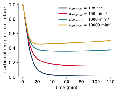

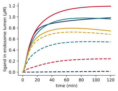
(a)

(b)

Figure 5.4: Receptor internalization and recycling with 0.1 nM ligand. (a) Receptors on the cell surface for several rates of ligand release in the endosome. (b) Ligand in the endosome lumen for the same cases. Total ligand (solid) reaches about 1 µM in the small lumen in every case, but the free fraction (dashed) depends on the rate of release. Receptors recycle only when release in the endosome is fast compared with their recapture by ligand.

Figure 5.4 shows what happens. With the medium at 0.1 nM, ligand-bound receptors are internalized within minutes. If the acidic endosome speeds ligand release only modestly, to 1 min⁻¹, receptors do not return to the surface, and only 1% of them are there after two hours. The reason is the small size of the lumen. Ligand carried in with the receptors accumulates in a volume of 0.01 pL, where its total concentration reaches 1.0 µM, 9,841 times its concentration in the medium. With slow release most of this ligand stays bound to receptors, and only 1% of it is free. A receptor in the endosome that loses its ligand is captured again in two ways, by binding a free ligand from the lumen, at a rate of about 16 min⁻¹, and by binding the free site of a ligand already held by another receptor in the endosomal membrane, at about 65 min⁻¹. Both rates are far larger than the rate of recycling, 0.1 min⁻¹, so a receptor returns to the surface only if it remains free, and the fraction of internalized receptors that are free is set by the competition between release and recapture. With release at 1 min⁻¹, slower than recapture, only 1% of the internalized receptors are free. With \(k_\mathrm{off,endo}\) = 10⁴ min⁻¹, release is faster than recapture (about 832 min⁻¹, now almost entirely by free ligand), 92% of the internalized receptors are free, and 50% of all receptors are on the surface after two hours.

The lumped endosome of this model exaggerates the effect, since a real cell has many small endosomes that mature, fuse, and deliver their contents to lysosomes. However, the calculation demonstrates the general point that compartment size affects a model through every bimolecular rule that applies in the compartment, including rules written with another compartment in mind. A universal rule should be checked in every compartment where it can apply, by reading the generated network.

5.7 Common mistakes

1. Scaling twice. Rate constants copied from a model with one rule per location, or fitted separately for each location, usually include the compartment size. Divide it out before using the constant in a universal rule.
2. Inconsistent surface sizes. Every surface must use the same effective thickness, and the size of a surface must be an area times that thickness, not an area alone.
3. Rules that reach too far. A universal rule applies in every compartment where its reactants can meet. Read the generated network for reactions in compartments you did not have in mind, as with ligand rebinding in the endosome above.
4. Overlapping transport rules. If two transport rules match the same complex, both apply and their rates add. For example, a complex that contains both a receptor and a co-receptor is internalized twice as fast if each has its own internalization rule.
5. Observables without a location. An observable that names no compartment counts molecules everywhere. Name the compartment when the location matters, and convert counts to concentrations with the size of the right compartment.
6. Impossible topology. A complex can include only one surface and the two volumes beside it, and a membrane that receives complexes by endocytosis needs a lumen inside it. BioNetGen rejects models that violate these constraints.

5.8 Summary

• cBNGL declares compartments as a tree of alternating volumes and surfaces, with the size of each.
• The location of a molecule is written M()@C, and that of a whole complex @C::. A complex can span one surface and its two adjacent volumes.
• A rule that names no compartment applies wherever its reactants can meet. BioNetGen divides each bimolecular rate constant by the size of the compartment where the reaction occurs, so the rule’s rate constant is intrinsic.
• Giving sizes as NAV, the number of molecules per µM, makes amounts numbers of molecules and keeps rate constants in concentration units.
• Transport rules move single molecules or whole complexes. Surface-to-surface species transport describes endocytosis.
• With nuclear transport, the STAT model shows nuclear accumulation of pSTAT and its reversal by SOCS feedback. With endocytosis, a small endosome concentrates released ligand enough to trap internalized receptors.

5.9 Exercises

1. Location as a state. Rewrite two_volumes.bngl without compartments, giving A and B a component loc~cp~nu. What rate constants must the two binding rules have to reproduce Figure 5.2? Check that the two models give identical trajectories.
2. Nuclear size. Vary V_NU in stat_compartments.bngl from 0.1 to 0.5 pL. How do the peak of nuclear pSTAT, measured in molecules and in concentration, and the adapted level of total pSTAT change? Explain which reactions are responsible.
3. Constitutive import. Some STATs enter the nucleus without phosphorylation (Reich and Liu 2006). Set kimp0 to zero and compare the response with Figure 5.3. What does basal shuttling contribute to the response?
4. Ligand depletion. In internalization.bngl, lower Lconc to 0.01 nM and plot the ligand remaining in the medium. Explain why the cells deplete the medium at this dose and not at 0.1 nM. How does the result depend on V_EC, the volume of medium per cell?
5. Signaling from endosomes. Combine the two models of this chapter so that receptors are internalized and recycled and STAT can be phosphorylated by receptors on either membrane. Does internalization shorten or prolong the STAT response?
6. Two anchors. Add a co-receptor N(l) that binds a second site on the ligand and an internalization rule for complexes that contain N. Find the complexes that are internalized at the sum of two rates, and modify the rules so that every complex is internalized at a single rate.

5.10 Further reading

Harris et al. (2009) defines cBNGL, including its topology rules, volume scaling, and the four kinds of transport. Reich and Liu (2006) reviews the nuclear transport of STAT proteins. Lauffenburger and Linderman (1993) is the classic treatment of receptor binding and trafficking models.

Begitt, Andreas, Thomas Meyer, Mathias van Rossum, and Uwe Vinkemeier. 2000. “Nucleocytoplasmic Translocation of Stat1 Is Regulated by a Leucine-Rich Export Signal in the Coiled-Coil Domain.” Proceedings of the National Academy of Sciences of the USA 97 (19): 10418–23. https://doi.org/10.1073/pnas.190318397.

Harris, Leonard A., Justin S. Hogg, and James R. Faeder. 2009. “Compartmental Rule-Based Modeling of Biochemical Systems.” Proceedings of the 2009 Winter Simulation Conference, 908–19. https://doi.org/10.1109/WSC.2009.5429719.

Hoeve, Johanna ten, Maria de Jesus Ibarra-Sanchez, Yubin Fu, et al. 2002. “Identification of a Nuclear Stat1 Protein Tyrosine Phosphatase.” Molecular and Cellular Biology 22 (16): 5662–68. https://doi.org/10.1128/MCB.22.16.5662-5668.2002.

Lauffenburger, Douglas A., and Jennifer J. Linderman. 1993. Receptors: Models for Binding, Trafficking, and Signaling. Oxford University Press.

Reich, Nancy C., and Ling Liu. 2006. “Tracking STAT Nuclear Traffic.” Nature Reviews Immunology 6 (8): 602–12. https://doi.org/10.1038/nri1885.