A simulation answers one question: what does the model do for one set of parameters and one initial condition? Most questions about a model are of a different kind. We wish to know which parameters control a response, how the response depends on the strength of the stimulus, how quickly the system settles and whether it oscillates on the way, and whether it can settle in more than one state. The tools that answer these questions are older than rule-based modeling and apply to any model that can be written as a set of ODEs. In this chapter we apply them to the cytokine–STAT–SOCS model of Chapter 1, extending the exercise on the shape of the pSTAT pulse at the end of that chapter, and to a variant of the circuit with positive feedback that acts as a switch with memory.
NoteLearning goals
After this chapter you should be able to:
find the conservation laws of a reaction network and explain what they imply for its steady states;
compute a steady state and determine its stability from the eigenvalues of the Jacobian;
relate eigenvalues to the timescales and the damped oscillations of a response;
compute dose–response curves with parameter scans;
compute normalized sensitivity coefficients and use them to find the parameters that control a response;
recognize bistability and hysteresis, and trace them with a continuation scan.
7.1 Conservation laws
Consider the model stat_step6_feedback.bngl from Chapter 1. Its twelve species are not independent. Ligand, receptor, STAT, and the SOCS promoter are neither made nor destroyed, only moved from one complex to another, so the total amount of each is fixed by the initial conditions. bngsim finds these conservation laws from the stoichiometry matrix when it loads a model:
model = bngsim.Model.from_bngl(model_path("ch01", "stat_step6_feedback"))laws = model.conservation_lawsfor row, total inzip(np.array(laws["coefficients"]), laws["constants"]): terms = [(name if c ==1elsef"{c:g}{name}")for c, name inzip(row, model.species_names) if c !=0]print(" + ".join(terms), "=", total)
Each law is a combination of species whose total does not change, which is the statement that a left null vector of the stoichiometry matrix exists (Chapter 1). With 4 conservation laws, the state of the system is determined by 8 independent variables, and the remaining species follow from the totals. Conservation laws matter in two ways. First, they confine the system to the set of states that share its totals, so that the steady states available to it depend on the initial conditions only through the totals. Second, they make the Jacobian of the full system singular, which is why steady-state solvers work in the reduced space of independent variables.
The first point does not mean that every initial condition with the same totals reaches the same steady state, since a set of states with fixed totals can contain more than one steady state. Whether it does is a property of the particular model, which must be checked. For this model, we may start with the receptors already bound to ligand and the STAT already phosphorylated, at the same totals, and compare the result with the steady state reached from the usual initial condition (computed in the next section):
sim = bngsim.Simulator(model, method="ode")def steady_pSTAT(initial): model.reset()for name, value in initial.items(): model.set_concentration(name, value) d = sim.steady_state(method="newton").to_dict()return d["Sp()"] + d["LRSp()"] + d["GSp()"]print(f"free ligand and receptor: {steady_pSTAT({}):.5f} uM")print(f"bound, STAT active: "f"{steady_pSTAT({'L()': 9, 'R()': 0, 'LR()': 1, 'S()': 0, 'Sp()': 10}):.5f} uM")
free ligand and receptor:  0.32247 uM
bound, STAT active:        0.32247 uM
The two agree, and so does every other initial condition with these totals that we have tried. In Section 7.5, by contrast, we will meet a model in which two initial conditions at the same parameters reach different steady states.
7.2 Steady states and their stability
A steady state is a state at which every rate of change is zero. The simplest way to find one is to simulate until nothing changes, and bngsim does this, followed by a Newton iteration that refines the result:
The steady state is the adapted level of Chapter 1. Whether the system actually returns to it after a small disturbance is a separate question, which is answered by linearizing the equations about the steady state. Let \(\mathbf{x}^*\) be the steady state and \(\boldsymbol{\delta} = \mathbf{x} - \mathbf{x}^*\) a small deviation. To first order,
where \(J\) is the Jacobian matrix. The solution is a sum of terms \(e^{\lambda t}\), one for each eigenvalue \(\lambda\) of \(J\). The Jacobian of the full system has a zero eigenvalue for each conservation law, which describes a change of the totals rather than a return to the steady state, so the eigenvalues that matter are those of the Jacobian of the independent variables. bngsim reports these. If every one of them has a negative real part, every small deviation decays and the steady state is locally stable. If any has a positive real part, some deviation grows and the steady state is unstable. If the largest real part is zero, the linear analysis is inconclusive.
The binding reaction of Chapter 1 shows how this works in the simplest case. With the two conservation laws, the state is determined by a single variable, \(x = [\mathrm{LR}]\), which obeys
and its single eigenvalue is negative for any concentrations, so the equilibrium is stable. A small deviation decays at the rate \(k_\mathrm{on}([\mathrm{L}] + [\mathrm{R}]) + k_\mathrm{off}\), which is the relaxation rate given in Chapter 1. Had we kept all three species as variables, the Jacobian would be a \(3\times3\) matrix with this eigenvalue and two zero eigenvalues, one for each conservation law. The STAT–SOCS model is treated the same way, with more variables.
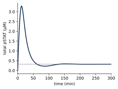
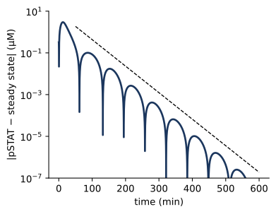
All 8 eigenvalues, one for each independent variable, have negative real parts, so the adapted state is stable. The real parts give the timescales of relaxation, \(\tau = -1/\mathrm{Re}\,\lambda\), and the imaginary parts give the frequencies of oscillation. The fastest mode decays with a time constant of 4 s, which is comparable to the time for a ligand-bound receptor to capture STAT, \(1/(k_\mathrm{Son}[\mathrm{S}]) \approx\) 6 s with 10 µM STAT, the fastest process in the model. The slowest pair of eigenvalues, -0.029 ± 0.050i min⁻¹, is complex. A complex pair describes a damped oscillation, with period \(2\pi/|\mathrm{Im}\,\lambda|\) = 127 min and decay time \(1/|\mathrm{Re}\,\lambda|\) = 34 min. This is the slow approach to the adapted level that we saw in Chapter 1, in which pSTAT undershoots and then recovers as SOCS overshoots and decays.
Figure 7.1: Relaxation to the adapted state is governed by the slowest eigenvalues. (a) Total pSTAT after stimulation (solid) and the steady state from the Newton solver (dashed). (b) Distance of pSTAT from its steady-state value on a logarithmic scale. At late times the envelope decays as \(e^{\mathrm{Re}\,\lambda\,t}\) for the slowest complex pair (dashed), and the dips mark the times at which the damped oscillation crosses the steady state.
Figure 7.1 b shows that this description is accurate well before the system reaches its steady state. After the first 50 min, the distance from the steady state shrinks along the envelope predicted by the slowest pair of eigenvalues, and it passes through zero roughly every half period.
7.3 Dose–response curves
The response of a cell to a signal depends on the strength of the signal, and a dose–response curve shows how. A parameter scan runs one simulation for each value of a parameter. bngsim provides it as a single call, which resets the initial state before each run:
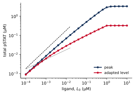
Figure 7.2: Dose–response curves of the cytokine–STAT–SOCS model. Peak and adapted levels of total pSTAT as functions of the initial ligand concentration. The dashed lines have slopes 1 and 1/2.
Figure 7.2 shows the peak and the adapted level of pSTAT over five decades of ligand concentration. Both saturate once the ligand exceeds the receptor concentration of 1 µM. Since the ligand binds tightly (\(K_D\) = 0.1 µM), nearly every ligand molecule finds a receptor until the receptors run out. Below saturation the two curves differ in shape. The peak grows in proportion to the dose (log–log slope 0.96 at the lowest doses), while the adapted level grows more slowly, with a slope of 0.62 in the middle of the range. The concentrations of ligand that give half of the maximal response, the EC₅₀ values, are 0.43 µM for the peak and 0.26 µM for the adapted level. Negative feedback thus compresses the adapted response. Between 0.001 and 0.1 µM ligand, a hundredfold range, the peak changes 60-fold and the adapted level only 16-fold. The next section explains where the square root comes from.
7.4 Sensitivity analysis
An exercise in Chapter 1 asked how doubling each parameter changes the time of the pSTAT peak, its height, and the adapted level. Sensitivity analysis makes this question systematic. The normalized sensitivity coefficient of an output \(y\) to a parameter \(p\) is
the percentage change in \(y\) per percentage change in \(p\) for small changes. A coefficient of 1 means that \(y\) is proportional to \(p\), a coefficient of −1 that it is inversely proportional, and a coefficient of 0 that \(p\) has no effect. Normalized coefficients have no units, so they can be compared across parameters of different kinds. For example, when ligand is in large excess over receptor, the fraction of receptors bound at equilibrium is \(y = [\mathrm{L}]/([\mathrm{L}] + K_D)\). Since \(\ln y = \ln [\mathrm{L}] - \ln([\mathrm{L}] + K_D)\), the sensitivity to the dissociation constant is \(S_{K_D}^y = -K_D/([\mathrm{L}] + K_D)\). With 1 µM ligand and \(K_D\) = 0.1 µM, \(S_{K_D}^y \approx -0.09\), so a 10% increase in \(K_D\) lowers the fraction bound by about 0.9%. The sensitivity is −1/2 when \([\mathrm{L}] = K_D\), and it approaches −1 at low ligand, where the fraction bound is proportional to \(1/K_D\). The idea goes back to metabolic control analysis, in which Heinrich and Rapoport, and independently Kacser and Burns, asked how the flux through a metabolic pathway is shared among its enzymes (Heinrich and Rapoport 1974).
We compute the coefficients for the three properties of the pulse by central differences, changing each parameter by ±1%. The time of the peak is found by fitting a parabola through the three highest points of the simulated curve, so that it is not limited by the spacing of the output times.
Code
def pulse(): model.reset() res = sim.run(t_span=(0, 600), n_points=6001) y, t = res.observables["pSTAT"], res.time i = np.argmax(y) a, b, c = np.polyfit(t[i-1:i+2], y[i-1:i+2], 2) t_peak =-b / (2* a)return np.array([t_peak, c - b**2/ (4* a), y[-1]])base = pulse()params =list(model.primary_param_names)S = {}h =0.01for name in params: v = model.get_param(name) model.set_param(name, v * (1+ h)); up = pulse() model.set_param(name, v * (1- h)); down = pulse() model.set_param(name, v) S[name] = (np.log(up) - np.log(down)) / (np.log(1+ h) - np.log(1- h))order =sorted(params, key=lambda n: -abs(S[n][2]))y = np.arange(len(order))fig, ax = plt.subplots(figsize=(6.0, 4.6))w =0.27for k, (label, color) inenumerate([("time of peak", "#5B6770"), ("peak height", "#1F7A8C"), ("adapted level", "#C8102E")]): ax.barh(y + (k -1) * w, [S[n][k] for n in order], height=w, color=color, label=label)ax.set_yticks(y)ax.set_yticklabels(order, fontsize=8)ax.invert_yaxis()ax.axvline(0, color="black", lw=0.6)ax.set_xlabel("normalized sensitivity")ax.legend(loc="lower right", fontsize=8)plt.show()# steady-state sensitivities from the solver, for comparisonmodel.reset()ss_s = sim.steady_state(method="newton", sensitivity_params=params)k_obs = ss_s.observable_names.index("pSTAT")S_ss = {n: ss_s.sensitivities_observables[k_obs][j] * model.get_param(n) / base[2]for j, n inenumerate(params)}initial = [n for n in params if n.endswith("0")]rates = [n for n in params if n notin initial]max_diff =max(abs(S_ss[n] - S[n][2]) for n in rates)half = [n for n in params ifabs(abs(S[n][2]) -0.5) <0.05]tmax =max(abs(S[n][0]) for n in params)
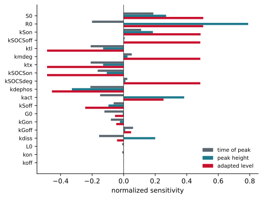
Figure 7.3: Normalized sensitivities of the pSTAT pulse to each parameter of the cytokine–STAT–SOCS model, computed by central differences with ±1% changes. Parameters are ordered by their effect on the adapted level.
Figure 7.3 shows the result. The three properties of the pulse depend on the parameters in different ways. The height of the peak depends most on the amount of receptor and on the rates of STAT phosphorylation and dephosphorylation, as one would expect for the early, feedback-free part of the response. The time of the peak is moderately sensitive to many parameters, none with a coefficient larger than 0.21 in magnitude. It is set by the race between the rise of pSTAT and the accumulation of SOCS, so it depends both on the parameters of the feedback loop and on those that make pSTAT rise faster, such as the amount of receptor. For the rate constants, the steady-state sensitivities computed by the solver, which differentiates the steady-state equations directly, agree with the finite-difference values for the adapted level to within 1e-05. The initial amounts are an exception. They affect the steady state only through the totals of the conservation laws, and the solver’s parameter sensitivities hold those totals fixed, so for the initial amounts the finite-difference values are the correct ones.
For the adapted level, 10 of the 19 parameters have coefficients close to +1/2 or −1/2. Consider the feedback loop at the adapted state, where nearly all ligand-bound receptors carry SOCS. The rate of STAT phosphorylation is proportional to the small fraction of receptors without SOCS, which is inversely proportional to the amount of SOCS. The amount of SOCS, in turn, is proportional to pSTAT, since the promoter is far from saturated and SOCS is made at a rate proportional to the occupied promoter. Setting production of pSTAT equal to its removal therefore gives an equation of the form \([\mathrm{pSTAT}] \propto A/[\mathrm{SOCS}] \propto A/[\mathrm{pSTAT}]\), where \(A\) collects the parameters that favor signaling. The adapted level is thus proportional to \(\sqrt{A}\), and every parameter that enters \(A\) or the SOCS–pSTAT proportionality as a simple factor has a sensitivity of ±1/2. The argument rests on three conditions, that SOCS occupies nearly all ligand-bound receptors, that the promoter is far from saturation, and that production and removal are linear in the relevant species. At the adapted state of this model, SOCS occupies 96% of the ligand-bound receptors and pSTAT occupies 14% of the promoters, so the first two conditions hold, and the other reactions of the model are first order or bimolecular with one partner in excess. The same argument explains the square-root dependence on dose in Figure 7.2, over the range of doses in which the conditions hold. Under these conditions, the negative feedback loop halves the sensitivity of the adapted state to most of its parameters, which is one way in which feedback can make a response less sensitive to variation in the amounts of its components.
Local sensitivities describe the effect of small changes around one set of parameter values. They can change sign or magnitude elsewhere in parameter space, and they say nothing about combinations of large changes. Global methods, which sample the whole range of plausible parameter values, and the related question of which parameters can be determined from data are taken up in Part III.
7.5 Switches and memory
Negative feedback, as in the STAT–SOCS loop, can make a response less sensitive to its parameters, although with delays it can also produce oscillations. Positive feedback can create two stable states, so that a cell responds to a graded signal with an all-or-none switch. Ferrell and Machleder found such a switch in the maturation of Xenopus oocytes, where individual oocytes respond to progesterone in an all-or-none fashion because the MAPK cascade is embedded in a positive feedback loop (Ferrell and Machleder 1998). Xiong and Ferrell later showed that the same loop gives the oocytes a memory, keeping the cascade active after the stimulus is removed (Xiong and Ferrell 2003).
A positive feedback loop is present in JAK–STAT signaling as well, since the gene for STAT1 is itself induced by STAT1. stat_autoloop.bngl is a minimal model of this loop. Receptor activity enters as the rate constant of STAT phosphorylation, kact, and STAT is made at a rate that is a Hill function of pSTAT, using a functional rate law (Chapter 4):
To map the steady states as a function of the signal, we use a continuation scan, bifurcate. Unlike a parameter scan, it does not reset the state between points. Each run starts from the end of the previous one, so the scan follows a branch of steady states as the parameter changes. Scanning kact up and then down reveals whether the branch depends on the direction of the scan.
Code
auto = bngsim.Model.from_bngl(model_path("ch07", "stat_autoloop"))asim = bngsim.Simulator(auto, method="ode")k_values = np.logspace(-2, 0, 41)auto.set_param("kact", k_values[0])auto.reset()up = asim.bifurcate("kact", list(k_values), t_span=(0, 5000), n_points=3)down = asim.bifurcate("kact", list(k_values[::-1]), t_span=(0, 5000), n_points=3)S_up = np.array([res.observables["STAT"][-1] for res in up])S_down = np.array([res.observables["STAT"][-1] for res in down])[::-1]k_on = k_values[np.argmax(S_up >2)]k_off = k_values[np.argmax(S_down >2)]# Exact steady states. At steady state pSTAT = kact*S0/(kdephos + kdeg) and# synthesis balances degradation, fsyn(pSTAT) = kdeg*STAT, so each value of# pSTAT gives one value of kact and of total STAT, including on the unstable# branch, which no forward simulation converges to.P = {k: auto.get_param(k) for k in ["kdephos", "ksyn0", "vmax", "K", "n", "kdeg"]}sp = np.logspace(-3, 1.5, 3000)fsyn = P["ksyn0"] + P["vmax"] * sp**P["n"] / (P["K"]**P["n"] + sp**P["n"])ratio = fsyn / (P["kdeg"] * sp) -1keep = ratio >0k_branch = (P["kdephos"] + P["kdeg"]) / ratio[keep]sp, S_branch = sp[keep], fsyn[keep] / P["kdeg"]stable = []for k, p_ss, S_ss inzip(k_branch, sp, S_branch): auto.set_param("kact", k) J = np.asarray(auto.jacobian(np.array([S_ss - p_ss, p_ss]))) stable.append(np.linalg.eigvals(J).real.max() <0)stable = np.array(stable)turn = np.where(np.diff(np.sign(np.diff(k_branch))) !=0)[0] +1k_fold_off, k_fold_on =sorted(k_branch[turn])fig, ax = plt.subplots(figsize=(4.2, 3.2))in_range = (k_branch > k_values[0]) & (k_branch < k_values[-1])for mask, style in [(stable, "-"), (~stable, "--")]: ax.semilogx(np.where(mask & in_range, k_branch, np.nan), S_branch, style, color="0.4", lw=1)ax.semilogx(k_values, S_up, "o", ms=4, label="increasing")ax.semilogx(k_values, S_down, "x", ms=5, label="decreasing")ax.axvspan(k_fold_off, k_fold_on, color="#D39B1E", alpha=0.15, lw=0)ax.set_xlabel("receptor activity, kact (min⁻¹)")ax.set_ylabel("steady-state STAT (µM)")ax.legend(loc="upper left")plt.show()# memory: hold kact = 0.3, apply a strong pulse, return to 0.3auto.set_param("kact", 0.3)auto.reset()seg1 = asim.run(t_span=(0, 100), n_points=101)auto.set_param("kact", 1.0)seg2 = asim.run(t_span=(100, 160), n_points=61)auto.set_param("kact", 0.3)seg3 = asim.run(t_span=(160, 500), n_points=341)t_all = np.concatenate([seg1.time, seg2.time, seg3.time])s_all = np.concatenate([seg1.observables["STAT"], seg2.observables["STAT"], seg3.observables["STAT"]])auto.set_param("kact", 0.1)fig, ax = plt.subplots(figsize=(4.2, 3.2))ax.axvspan(100, 160, color="#D39B1E", alpha=0.2, lw=0)ax.plot(t_all, s_all)ax.set_xlabel("time (min)")ax.set_ylabel("total STAT (µM)")plt.show()# stability of each branch at kact = 0.3, from the eigenvalues of the Jacobiandef eigenvalues_at(state):return np.linalg.eigvals(np.asarray(auto.jacobian(np.asarray(state))))auto.set_param("kact", 0.3)auto.reset()asim.run(t_span=(0, 5000), n_points=3)eig_low = eigenvalues_at(auto.get_state())auto.set_state(np.array([1.0, 9.0])) # start near the upper branchasim.run(t_span=(0, 5000), n_points=3)eig_high = eigenvalues_at(auto.get_state())auto.set_param("kact", 0.1)max_re =max(np.real(eig_low).max(), np.real(eig_high).max())
(a)
(b)
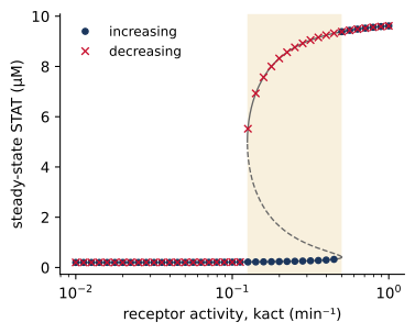
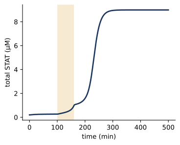
Figure 7.4: A positive feedback loop makes a switch with memory. (a) Steady-state STAT as a function of receptor activity, from continuation scans with increasing (circles) and decreasing (crosses) kact, and from the exact solution of the steady-state equations, with stable (solid) and unstable (dashed) branches. Between the two saddle-node bifurcations (shaded) the system is bistable. (b) A transient signal switches the system to the upper state. With kact held at 0.3 min⁻¹ inside the bistable range, a 60-min pulse of strong signal (shaded) moves the system to the upper state, where it remains after the signal returns to 0.3.
Figure 7.4 a shows the result. When the signal increases from a low value, STAT stays near its basal level until kact reaches about 0.50 min⁻¹, and then jumps to a level about 48 times higher. When the signal decreases from a high value, STAT stays high until kact falls below about 0.13 min⁻¹. Between these thresholds the system has two stable steady states, and which one it occupies depends on its history. This dependence on history is called hysteresis. The eigenvalues confirm that both states are stable, since at kact = 0.3 min⁻¹ the largest real part of any eigenvalue on either branch is -0.049 min⁻¹. Between the two stable states lies a third, unstable, steady state, which separates the initial conditions that go to one stable state from those that go to the other. A forward simulation does not converge to it, so a continuation scan cannot show it. For this two-species model, however, the steady-state equations can be solved exactly, and the solution traces all three branches in Figure 7.4 a. The thresholds are saddle-node bifurcations, the points at which the unstable state collides with one of the stable states and both disappear (Tyson et al. 2003). The exact solution places them at 0.125 and 0.500 min⁻¹. A continuation scan locates them only to within the spacing of its grid, and near a bifurcation it converges slowly, since the eigenvalue that governs the approach to the steady state passes through zero there. Thresholds from a scan should therefore be checked with a finer grid and longer runs, or, when the equations allow it, by solving for the steady states directly.
Figure 7.4 b shows the practical consequence. A cell that sees a moderate signal remains in the low state, but a transient strong signal moves it to the high state, where it stays after the signal returns to its moderate level. In this deterministic model it stays there for as long as kact remains in the bistable range, and the circuit thus remembers the strong signal, as the oocytes of Xiong and Ferrell do. In a stochastic model, fluctuations can return the cell to the low state, although such transitions become rare as the numbers of molecules grow. Whether STAT1 autoregulation creates memory of this kind in real cells is not established by this model, which is deliberately minimal. The model does show what properties such a memory would require: feedback that is both strong and cooperative enough, here through a Hill coefficient of 2, to produce two stable states over the relevant range of signals.
7.6 Common mistakes
Stopping a simulation too early. A response that has not reached steady state can look flat on a linear scale. Check by plotting the distance from the steady state on a logarithmic scale, as in Figure 7.1, or use a steady-state solver.
Forgetting the conservation laws. The steady state depends on the totals of conserved quantities. Changing the initial amount of a species in a scan changes a total, and changing a species that is not in the seed species may have no effect at all.
Reading too much into local sensitivities. A sensitivity describes small changes around one point in parameter space and can be very different elsewhere.
Finite-difference steps of the wrong size. Steps that are too large give the sensitivity of a nonlinear function averaged over a range; steps that are too small are swamped by the numerical error of the solver. Changes of about 1% with tight solver tolerances are a reasonable starting point, and the solver’s own sensitivities avoid the problem.
Missing bistability. A parameter scan that resets the initial state for every point follows only one branch. Use a continuation scan in both directions, or start simulations from several initial conditions, whenever a model contains positive feedback.
7.7 Summary
Conservation laws reduce the number of independent variables and confine the system to states with fixed totals. Whether those totals determine a single steady state must be checked for each model.
A steady state is locally stable if all eigenvalues of the Jacobian of the independent variables have negative real parts. The real parts give the timescales of relaxation, and the imaginary parts of complex pairs give the periods of damped oscillations.
The slowest complex pair of the STAT–SOCS model accounts for the slow, oscillatory approach of pSTAT to its adapted level.
Parameter scans give dose–response curves. Negative feedback compresses the adapted response, which grows roughly as the square root of the dose.
Normalized sensitivity coefficients identify the parameters that control a response. The adapted pSTAT level has sensitivities of about ±1/2 to most parameters, a consequence of the feedback loop when SOCS occupies most receptors and the promoter is far from saturation.
Positive feedback can create two stable states. Continuation scans in both directions reveal hysteresis, and a transient signal can switch such a system to its upper state, where a deterministic model keeps it while the signal stays in the bistable range.
7.8 Exercises
Conservation laws. Find the conservation laws of stat_rbm1_rules.bngl from Chapter 2 with model.conservation_laws. How many are there, and how do they compare with those of the network model?
Timescales. Compute the eigenvalues at the adapted state of stat_step6_feedback.bngl as kSOCSdeg is varied from 0.01 to 0.5 min⁻¹. How do the period and decay time of the slowest mode change? Is there a value at which the oscillation becomes sustained?
Sensitivity of the peak. Explain from the structure of the model why increasing the amount of receptor raises the peak and makes it occur earlier, while increasing the rate of SOCS translation lowers the peak and also makes it occur earlier.
Testing the square-root law. Use the model to check the argument for the ±1/2 sensitivities. Plot the fraction of ligand-bound receptors carrying SOCS and the fraction of occupied promoters at the adapted state as functions of L0. Where does the argument break down, and how do the sensitivities change there?
Removing the switch. Repeat Figure 7.4 a with Hill coefficients n = 1, 1.5, and 3. For which values is there a bistable range? How does its width depend on n?
Global sensitivity. Draw 200 sets of parameters for stat_step6_feedback.bngl, each parameter varied by a random factor between 1/3 and 3 on a logarithmic scale. Plot the adapted level against each parameter. Which parameters still stand out, and does the square-root pattern survive?
7.9 Further reading
Tyson et al. (2003) is an accessible introduction to the dynamics of signaling motifs, including switches and oscillators, and Tyson and Novák (2010) extends it. Ferrell and Machleder (1998) and Xiong and Ferrell (2003) are the classic experimental studies of a bistable switch with memory. Heinrich and Rapoport (1974) introduced the sensitivity coefficients of metabolic control analysis.
Ferrell, James E., and Eric M. Machleder. 1998. “The Biochemical Basis of an All-or-None Cell Fate Switch in Xenopus Oocytes.”Science 280 (5365): 895–98. https://doi.org/10.1126/science.280.5365.895.
Heinrich, Reinhart, and Tom A. Rapoport. 1974. “A Linear Steady-State Treatment of Enzymatic Chains. General Properties, Control and Effector Strength.”European Journal of Biochemistry 42 (1): 89–95. https://doi.org/10.1111/j.1432-1033.1974.tb03318.x.
Tyson, John J., Katherine C. Chen, and Béla Novák. 2003. “Sniffers, Buzzers, Toggles and Blinkers: Dynamics of Regulatory and Signaling Pathways in the Cell.”Current Opinion in Cell Biology 15 (2): 221–31. https://doi.org/10.1016/S0955-0674(03)00017-6.
Xiong, Wen, and James E. Ferrell. 2003. “A Positive-Feedback-Based Bistable ‘Memory Module’ That Governs a Cell Fate Decision.”Nature 426 (6965): 460–65. https://doi.org/10.1038/nature02089.