Every simulation method in Part I begins by generating the reaction network implied by the rules. For the models of Chapter 2 this is quick, since the networks contain at most a few hundred reactions. For many models of signaling, however, the network is too large to generate, and for some it is infinite. Chapter 4 showed one example. A ligand with two binding sites and a receptor with two sites form chains of any length, and the network grows without limit unless the size of complexes is capped. Hlavacek and coworkers reviewed this combinatorial explosion, which they called the “complexity of complexes,” and argued for models built from molecular domains rather than lists of species (Hlavacek et al. 2003). In this chapter we describe how a rule-based model can be simulated without generating its network, use the method to study the aggregation of receptors by a trivalent ligand, and discuss when network-free simulation is and is not the right choice.
NoteLearning goals
After this chapter you should be able to:
explain why the network generated from a set of rules can be too large to use, and recognize models where this happens;
describe how a network-free simulator applies rules directly to individual molecules;
run network-free simulations with bngsim and analyze the complexes they produce;
verify a network-free simulation against a network-based method;
choose between network-based and network-free methods for a given model.
6.1 Rules without a network
Consider the stochastic simulation algorithm of Chapter 3. At each step it uses the propensity of every reaction, computed from the numbers of molecules of each species, chooses a reaction with probability proportional to its propensity, and updates the species counts. Efficient implementations recompute only the propensities that the last reaction changed, but the cost of a step still grows with the size of the network, and the list of reactions must be known in advance.
A network-free simulator applies the same logic to rules instead of reactions. The state of the system is a collection of individual molecules, each with its components, states, and bonds, and a complex is a set of molecules connected by bonds. The simulator proceeds as follows:
For each rule, it keeps a list of the molecules (or groups of molecules) that match each reactant pattern. The propensity of the rule is its rate constant times the number of ways the rule can be applied, which for a bimolecular rule is the product of the lengths of the two lists, corrected for symmetry.
It chooses the time of the next event from the total propensity of all rules and chooses a rule with probability proportional to its propensity, just as Gillespie’s algorithm chooses a reaction.
It picks reactants at random from the lists of the chosen rule and checks any conditions that the lists do not capture, for example that two reactants of a + rule belong to different complexes. If a condition fails, nothing happens, and the step is a null event.
Otherwise it applies the rule, changing bonds and states of the chosen molecules, and updates the lists for the molecules that changed and their neighbors.
Since the simulator never enumerates species or reactions, the cost of a step depends on the number of rules and on the size of the neighborhood that a rule changes, but not on the size of the network. Memory grows with the number of molecules rather than the number of species. The price is that every simulation is stochastic and tracks each molecule, so the cost grows with the number of molecules and the number of events, and, as we will see, with the size of the complexes.
The first network-free simulators appeared at about the same time. Danos, Feret, Fontana, and Krivine developed a scalable method for the Kappa language (Danos et al. 2007), and Yang, Monine, Faeder, and Hlavacek introduced a kinetic Monte Carlo method for BNGL, which they used to study multivalent ligand–receptor binding (Yang et al. 2008). Colvin and coworkers then wrote RuleMonkey, which implements an exact method that avoids null events (Colvin et al. 2010), and Michael Sneddon, the author, and Thierry Emonet wrote NFsim, which is designed for large models and supports functional rate laws (Sneddon et al. 2011). bngsim includes both NFsim and RuleMonkey.
6.2 Running a network-free simulation
Network-free simulators read the rules of a model from an XML file that BioNetGen writes with the action writeXML(). The model file itself needs no changes. In BNGL, the action simulate({method=>"nf"}) writes the XML file and runs NFsim in one step. In Python, bngsim provides a session object that loads the XML file and runs the simulation:
xml = bng_xml("ch03", "stat_ssa_feedback") # runs BioNetGen's writeXML()with bngsim.NfsimSession(str(xml)) as nf: nf.initialize(seed=1) result = nf.simulate(0, 240, n_points=49)
The session returns the same Result object as the network-based methods, with the observables of the model as functions of time. Since NFsim tracks individual molecules, amounts must be numbers of molecules, as for the SSA, and rate constants must be in per-molecule units (Chapter 3).
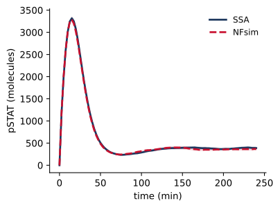
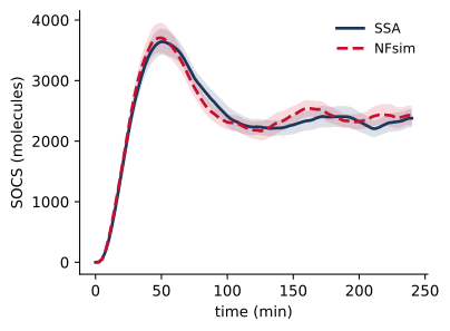
The first test of any network-free simulation is a model whose network is small enough to simulate both ways. The stochastic STAT–SOCS model of Chapter 3 is such a model. Figure 6.1 compares averages over many runs of NFsim and of the SSA.
Code
n_runs =40model = bngsim.Model.from_bngl(model_path("ch03", "stat_ssa_feedback"))ssa = bngsim.Simulator(model, method="ssa")model.reset()t0 = time.perf_counter()ssa_runs = ssa.run_replicates(n_runs, t_span=(0, 240), n_points=97, seed=1)t_ssa = time.perf_counter() - t0xml =str(bng_xml("ch03", "stat_ssa_feedback"))t0 = time.perf_counter()nf_runs = []for seed inrange(1, n_runs +1):with bngsim.NfsimSession(xml) as nf: nf.initialize(seed=seed) nf_runs.append(nf.simulate(0, 240, n_points=97))t_nf = time.perf_counter() - t0t = ssa_runs[0].timewithin = {}for obs, label in [("pSTAT", "pSTAT (molecules)"), ("SOCS", "SOCS (molecules)")]: a = np.array([r.observables[obs] for r in ssa_runs]) b = np.array([r.observables[obs] for r in nf_runs]) se_a = a.std(0, ddof=1) / np.sqrt(n_runs) # standard error of each mean se_b = b.std(0, ddof=1) / np.sqrt(n_runs)# fraction of time points (after t = 0) at which the two means differ by# less than two standard errors of their difference z = np.abs(a.mean(0) - b.mean(0))[1:] / np.sqrt(se_a**2+ se_b**2)[1:] within[obs] = np.mean(z <2) fig, ax = plt.subplots(figsize=(4.2, 3.2))for x, se, style, name in [(a, se_a, "-", "SSA"), (b, se_b, "--", "NFsim")]: line, = ax.plot(t, x.mean(0), style, label=name) ax.fill_between(t, x.mean(0) -2* se, x.mean(0) +2* se, color=line.get_color(), alpha=0.15, lw=0) ax.set_xlabel("time (min)") ax.set_ylabel(label) ax.legend(loc="upper right") plt.show()
(a)
(b)
Figure 6.1: A network-free simulation agrees with a network-based one. Mean total pSTAT (a) and SOCS (b) from 40 stochastic simulations of the STAT–SOCS model of Chapter 3 with the SSA (solid) and with NFsim (dashed). Shaded bands show two standard errors of each mean.
The two methods agree to within the statistical error of the averages. At 99% of the time points for pSTAT and 97% for SOCS, the two means differ by less than two standard errors of their difference, about the 95% expected if the two methods sample the same process. They are not equally fast, however. On the computer that built this book, the 40 NFsim runs of this model took 12.4 s and the 40 SSA runs took 0.4 s, a factor of 32. For a network as small as this one, following individual molecules costs more than updating the counts of a few dozen species, and the network-based method is the better choice. Timings like these depend on the computer, the software versions, and the model, so they should be measured for the model at hand.
6.3 Receptor aggregation and the sol–gel transition
Consider now a model whose network cannot be generated. Many immune receptors, such as the high-affinity IgE receptor FcεRI on mast cells, signal when a multivalent antigen crosslinks them into aggregates. Goldstein and Perelson studied the simplest model that produces large aggregates, a ligand with three identical binding sites and a receptor with two (Goldstein and Perelson 1984). They showed that when crosslinking is strong enough, there is a range of ligand concentrations in which most receptors join a single aggregate whose size is limited only by the number of receptors on the cell. This is a sol–gel phase transition, like the one that turns a solution of polymers into a gel.
tlbr.bngl contains three rules: binding of free ligand to a receptor, and crosslinking by a ligand that already has one or two sites bound.
# Free ligand binds a receptor siteFreeBind: L(r,r,r) + R(l) <-> L(r!1,r,r).R(l!1) kp1, koff# A ligand with one or two sites bound captures another receptorCross1: L(r!+,r,r) + R(l) <-> L(r!+,r!1,r).R(l!1) kp2, koffCross2: L(r!+,r!+,r) + R(l) <-> L(r!+,r!+,r!1).R(l!1) kp2, koff
The + in the crosslinking rules means that the ligand and the receptor must belong to different complexes, so the rules do not close rings. The binding rate constants are set by two dimensionless parameters introduced by Goldstein and Perelson, a ligand concentration \(c = 3 k_{p1} L_\mathrm{tot}/k_\mathrm{off}\) and a crosslinking constant \(\beta = k_{p2} R_\mathrm{tot}/k_\mathrm{off}\). In the scans below we change \(c\) by changing \(k_{p1}\), with the number of ligands fixed at 4200. Since each ligand has three sites and there are only 600 receptor sites, at most one ligand in seven can be bound, and the free ligand stays within 15% of the total. Changing \(k_{p1}\) at fixed ligand is therefore nearly equivalent to changing the amount of ligand at fixed affinity, which is what an experiment does, and the theory, which assumes that binding does not deplete the ligand, applies with small corrections.
These three rules generate an infinite network. Table 6.1 shows the network generated when complexes are limited to max_agg molecules, together with the time BioNetGen takes to generate it.
Table 6.1: Size of the network generated from tlbr.bngl as a function of max_agg, the largest complex allowed, and the time for bngsim to load the model, which includes parsing, network generation, and preparation for simulation.
species
reactions
time (s)
max_agg
3
5
6
0.2
5
10
28
0.2
7
19
92
1.0
9
36
280
8.2
The number of species grows slowly, but on the computer that built this book the time to load the model grows by a factor of about 3 for each molecule added to the largest complex. Part of the cost is that every complex a rule produces must be compared with the species already found to decide whether it is new, and the number of ways the rules can be applied grows with the size of the complexes. At this rate, a network that includes a gel of hundreds of molecules is far out of reach.
Code
xml =str(bng_xml("ch06", "tlbr"))Rtot =300koff =0.01c_values = [0.001, 0.01, 0.1, 0.84, 3, 10, 30, 100]def t_equil(c):# Free ligand binds a receptor site at rate c*koff/3, so equilibration is# slow at low c. These run lengths were checked against longer runs.returnmax(1e4, 1.5/ (c * koff))largest, largest_se, bonds_nf, drift = [], [], [], []species_file = os.path.join(tempfile.gettempdir(), "tlbr_final.species")for c in c_values: frac, b, b_half = [], [], []for seed in [1, 2, 3]:with bngsim.NfsimSession(xml) as nf: nf.set_param("cTot", c) nf.initialize(seed=seed) r = nf.simulate(0, t_equil(c), n_points=3) # t = 0, t_end/2, t_end nf.save_species(species_file) frac.append(aggregate_sizes(species_file, "R").max() / Rtot) b.append(r.observables["Bonds"][-1]) b_half.append(r.observables["Bonds"][1]) largest.append(np.mean(frac)) largest_se.append(np.std(frac, ddof=1) / np.sqrt(len(frac))) bonds_nf.append(np.mean(b)) drift.append(abs(np.mean(b) - np.mean(b_half)) / np.mean(b))# the same runs at c = 0.01, stopped early at 2000 searly = []for seed in [1, 2, 3]:with bngsim.NfsimSession(xml) as nf: nf.set_param("cTot", 0.01) nf.initialize(seed=seed) nf.simulate(0, 2000, n_points=2) nf.save_species(species_file) early.append(aggregate_sizes(species_file, "R").max() / Rtot)early = np.mean(early)# network-based ODEs with complexes capped at eight moleculeswith tempfile.TemporaryDirectory() as d: path = os.path.join(d, "tlbr8.bngl")open(path, "w").write(src +"\ngenerate_network({overwrite=>1,max_agg=>8})\n") m8 = bngsim.Model.from_bngl(path)ode8 = bngsim.Simulator(m8, method="ode")c_fine = np.logspace(-3, 2, 31)bonds_ode = []for c in c_fine: m8.set_param("cTot", c) m8.reset() bonds_ode.append(ode8.run(t_span=(0, 10* t_equil(c)), n_points=3).observables["Bonds"][-1])fig, ax = plt.subplots(figsize=(4.2, 3.2))ax.errorbar(c_values, largest, yerr=largest_se, fmt="o-", capsize=2)ax.set_xscale("log")ax.set_xlabel("ligand concentration, $c$")ax.set_ylabel("fraction of receptors\nin largest aggregate")ax.set_ylim(0, 1)plt.show()fig, ax = plt.subplots(figsize=(4.2, 3.2))ax.semilogx(c_fine, np.array(bonds_ode) / Rtot, "-", color="#5B6770", label="ODE, max_agg = 8")ax.semilogx(c_values, np.array(bonds_nf) / Rtot, "o", label="NFsim")ax.set_xlabel("ligand concentration, $c$")ax.set_ylabel("bonds per receptor")ax.set_ylim(0, 2.05)ax.legend(loc="lower right")plt.show()i84 = c_values.index(0.84)ode_at = np.interp(np.log(c_values), np.log(c_fine), bonds_ode)err =1- ode_at / np.array(bonds_nf) # relative error of the capped ODEserr84 = err[i84]
(a)
(b)
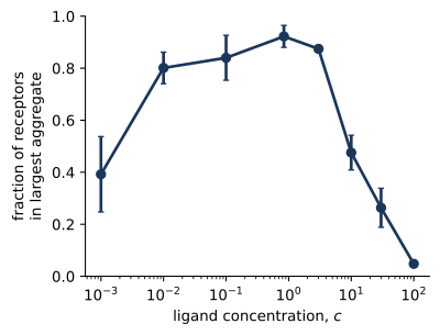
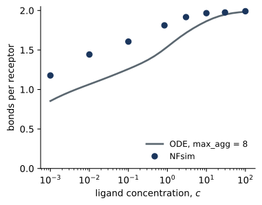
Figure 6.2: The sol–gel transition in the TLBR model with \(\beta\) = 50, simulated with NFsim. (a) Fraction of receptors in the largest aggregate at equilibrium as a function of the dimensionless ligand concentration c, with the standard error of the mean of three runs. (b) Ligand–receptor bonds from NFsim (points) and from the ODEs for the network with aggregates capped at eight molecules (line).
Figure 6.2 shows the transition. Over a wide range of ligand concentrations, a single aggregate forms that contains most of the receptors, for example 92% of them at \(c\) = 0.84. Since the simulation contains only 300 receptors, the size of the gel is limited by the size of the system, which is the finite-cell analog of the infinite aggregate of the theory. At high concentration each receptor site is occupied by a different ligand, and the largest aggregate shrinks to 5% of the receptors at \(c\) = 100. At low concentration there is too little ligand to link the receptors, but with strong crosslinking the gel persists to low doses, and at \(c\) = 0.001 the largest aggregate still contains 39% of them.
Each point in Figure 6.2 is an equilibrium value, and reaching equilibrium takes much longer at low concentration, since a free ligand binds a receptor site only at the rate \(c\,k_\mathrm{off}/3\), which is once every 3×10⁵ s at \(c\) = 0.001. A run that stops too early underestimates the aggregates. At \(c\) = 0.01, for example, runs stopped at 2000 s, which is long enough at high concentration, give a largest aggregate of 10% of the receptors rather than 80%. The runs here last at least 10⁴ s and longer at low concentration, and the mean number of bonds changes by at most 3% over the second half of each run. Since NFsim is stochastic, each point is the mean of three runs, and the error bars show its standard error. The scatter is largest at the edges of the gel phase, where the size of the largest aggregate fluctuates widely in time.
The network capped at eight molecules gives the wrong answer in this range. At \(c\) = 0.84 it underestimates the number of ligand–receptor bonds by 17%, because the cap forbids the aggregates that the system actually forms. At \(c\) = 100, where aggregates are small, the capped network and NFsim differ by 0.3%, but at \(c\) = 0.001, where large aggregates remain, the cap still causes an error of 27%. It is important to note that the size of this error cannot be known in advance. The only way to check that a cap is adequate is to compare with a larger cap or with a network-free simulation, as recommended in Chapter 4.
Monine and coworkers used network-free simulations of this kind to compare the TLBR model with measurements of a trivalent antigen binding IgE–FcεRI on mast cells (Monine et al. 2010). They found that the simple model predicts extensive aggregation at antigen doses where cells secrete strongly, and examined how steric constraints and the formation of rings would change the prediction. Such questions require keeping track of the structure of each aggregate, which a network-free simulation does automatically.
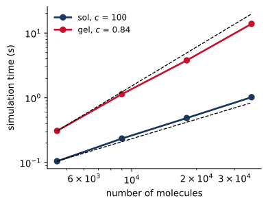
Figure 6.3: The cost of a network-free simulation depends on the size of the complexes as well as the number of molecules. Time to simulate 500 s of the TLBR model with NFsim, starting from free ligands and receptors, with the numbers of ligands and receptors multiplied by a common factor and \(\beta\) fixed, in the sol phase (c = 100) and in the gel phase (c = 0.84). The dashed lines have slopes 1 and 2.
Figure 6.3 shows how the cost of a network-free simulation grows with the size of the system. The rate of events grows in proportion to the number of molecules, and in the sol phase the cost of each event stays about the same, so the time to simulate a fixed interval grows linearly (the fitted slope is 1.1). In the gel phase the time grows about as the square of the number of molecules (slope 1.8) in these measurements. One expects faster than linear growth because the gel grows with the system, and some events require the simulator to traverse the whole complex that contains the reactants. When a bond in the gel breaks, for example, the simulator must determine whether the complex has split in two, and a + rule must check that its reactants belong to different complexes. Network-free simulation thus trades the cost of the network, which depends on the number of possible species, for a cost that depends on the molecules actually present and on how they are connected. Table 6.2 summarizes when each kind of method is the better choice.
Table 6.2: Choosing a simulation method.
Network-based (ODE, SSA, PSA)
Network-free (NFsim, RuleMonkey)
Requires
a finite network small enough to generate
rules only
Cost grows with
number of reactions
number of molecules and events
Results
deterministic (ODE) or stochastic
stochastic only
Suited to
small and medium networks, fitting, steady states, sensitivity analysis
large or infinite networks, aggregation, polymerization, large models with many sites
Information on complexes
counts of each species
the structure of every complex
A practical consequence is that a modeler can often use both kinds of methods on the same model. The BNGL file is the same, so a model can be developed and fitted with a network capped at a moderate size and then checked with a network-free simulation, or simulated network-free in the regime where the cap fails.
6.5 Common mistakes
Using network-free simulation by default. When the network is small, NFsim is much slower than the SSA, and an ODE solution may suffice. Use network-free methods when the network is large or infinite.
Too few runs. Network-free results are stochastic. Average over enough runs to make the statistical error smaller than the effect being studied, and report it.
Concentration units. As for the SSA, amounts must be numbers of molecules and rate constants must be per molecule (Chapter 3).
Rings formed by intermolecular rules. A + between reactant patterns means that the reactants are in different complexes. bngsim enforces this by default, but the standalone NFsim program does not unless it is given the -bscb option. Write ring closure as a separate unimolecular rule, as in Chapter 4.
Expensive observables.Species observables require the simulator to track whole complexes, which can slow a simulation with very large aggregates. Use Molecules observables where they suffice.
Unsupported features. Some BNGL features available to network-based methods, such as compartments (Chapter 5), are not supported by every network-free simulator. Check the documentation of the simulator before relying on them.
6.6 Summary
Rules for multivalent binding can generate networks that are too large to generate or infinite.
A network-free simulator applies rules directly to individual molecules, choosing events with the same probabilities as Gillespie’s algorithm, so its cost does not depend on the size of the network.
bngsim runs NFsim and RuleMonkey from the XML file that BioNetGen writes from the model, with no change to the model.
A network-free simulation agrees with the SSA, within statistical error, on a model with a small network, but for that model it is much slower.
The TLBR model shows a sol–gel transition in which most receptors join one aggregate. A capped network misses this behavior, while a network-free simulation captures it. Near the edges of the gel phase, and especially at low ligand concentration, equilibration is slow, and run lengths must be checked.
Network-based and network-free methods can be used on the same BNGL model. Choose by the size of the network and the questions being asked.
6.7 Exercises
RuleMonkey. Repeat Figure 6.1 with bngsim.RuleMonkeySession in place of NfsimSession. Do the results agree? Which is faster for this model and for TLBR?
Crosslinking strength. Repeat the scan of Figure 6.2 with β = 5 and β = 500, using run lengths long enough to reach equilibrium at every dose. How does the range of ligand concentrations in which a gel forms depend on β? Is there a value of β below which no gel forms? Compare your results with the theory of Goldstein and Perelson (1984).
Aggregate size distribution. At \(c\) = 0.01, 0.84, and 30, plot the distribution of the number of receptors per aggregate from the final species of an NFsim run. How does the distribution change across the transition?
When does a cap work? For \(c\) = 30, find the smallest max_agg for which the ODE solution for the number of bonds agrees with NFsim to within 2%. Repeat for \(c\) = 0.84. What does the difference tell you?
Rings. Add a unimolecular rule that lets a bound ligand bind a free receptor site in the same aggregate, with rate constant kring. Simulate with NFsim for several values of kring. How do rings affect the size of the largest aggregate? Compare with the discussion in Monine et al. (2010).
6.8 Further reading
Sneddon et al. (2011) describes NFsim, its algorithm, and its performance on large models. Yang et al. (2008) and Colvin et al. (2010) describe the kinetic Monte Carlo method and RuleMonkey. Danos et al. (2007) describes network-free simulation for the Kappa language. Goldstein and Perelson (1984) is the classic theory of aggregation by a trivalent ligand, and Monine et al. (2010) compares it with experiment.
Colvin, Joshua, Michael I. Monine, Ryan N. Gutenkunst, William S. Hlavacek, Daniel D. Von Hoff, and Richard G. Posner. 2010. “RuleMonkey: Software for Stochastic Simulation of Rule-Based Models.”BMC Bioinformatics 11: 404. https://doi.org/10.1186/1471-2105-11-404.
Danos, Vincent, Jérôme Feret, Walter Fontana, and Jean Krivine. 2007. “Scalable Simulation of Cellular Signaling Networks.”Programming Languages and Systems (APLAS 2007), Lecture notes in computer science, 139–57. https://doi.org/10.1007/978-3-540-76637-7_10.
Goldstein, Byron, and Alan S. Perelson. 1984. “Equilibrium Theory for the Clustering of Bivalent Cell Surface Receptors by Trivalent Ligands. Application to Histamine Release from Basophils.”Biophysical Journal 45 (6): 1109–23. https://doi.org/10.1016/S0006-3495(84)84259-9.
Hlavacek, William S., James R. Faeder, Michael L. Blinov, Alan S. Perelson, and Byron Goldstein. 2003. “The Complexity of Complexes in Signal Transduction.”Biotechnology and Bioengineering 84 (7): 783–94. https://doi.org/10.1002/bit.10842.
Monine, Michael I., Richard G. Posner, Paul B. Savage, James R. Faeder, and William S. Hlavacek. 2010. “Modeling Multivalent Ligand-Receptor Interactions with Steric Constraints on Configurations of Cell-Surface Receptor Aggregates.”Biophysical Journal 98 (1): 48–56. https://doi.org/10.1016/j.bpj.2009.09.043.
Sneddon, Michael W., James R. Faeder, and Thierry Emonet. 2011. “Efficient Modeling, Simulation and Coarse-Graining of Biological Complexity with NFsim.”Nature Methods 8 (2): 177–83. https://doi.org/10.1038/nmeth.1546.
Yang, Jin, Michael I. Monine, James R. Faeder, and William S. Hlavacek. 2008. “Kinetic Monte Carlo Method for Rule-Based Modeling of Biochemical Networks.”Physical Review E 78 (3): 031910. https://doi.org/10.1103/PhysRevE.78.031910.